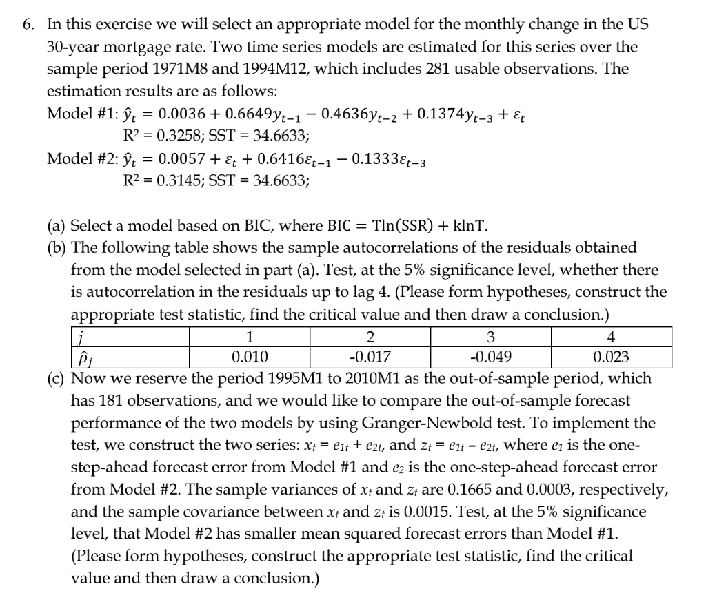
6. In this exercise we will select an appropriate model for the monthly change in the US 30-year mortgage rate. Two time series models are estimated for this series over the sample period 1971M8 and 1994M12, which includes 281 usable observations. The estimation results are as follows: Model #1: yt = 0.0036 + 0.6649yt-1 0.4636yt-2 + 0.1374yt-3 + t R2 = 0.3258; SST = 34.6633; Model #2: t = 0.0057 + &t + 0.6416t-1 0.1333&t-3 R2 = 0.3145; SST = 34.6633; 3 (a) Select a model based on BIC, where BIC = Tln(SSR) + klnt. (b) The following table shows the sample autocorrelations of the residuals obtained from the model selected in part (a). Test, at the 5% significance level, whether there is autocorrelation in the residuals up to lag 4. (Please form hypotheses, construct the appropriate test statistic, find the critical value and then draw a conclusion.) 1 2. 4 | 0.010 -0.017 -0.049 0.023 (c) Now we reserve the period 1995M1 to 2010M1 as the out-of-sample period, which has 181 observations, and we would like to compare the out-of-sample forecast performance of the two models by using Granger-Newbold test. To implement the test, we construct the two series: X+ = 21+ + eat, and zz = C1t - ezt, where ei is the one- step-ahead forecast error from Model #1 and e2 is the one-step-ahead forecast error from Model #2. The sample variances of x; and z are 0.1665 and 0.0003, respectively, and the sample covariance between xt and zt is 0.0015. Test, at the 5% significance level, that Model #2 has smaller mean squared forecast errors than Model #1. (Please form hypotheses, construct the appropriate test statistic, find the critical value and then draw a conclusion.) 6. In this exercise we will select an appropriate model for the monthly change in the US 30-year mortgage rate. Two time series models are estimated for this series over the sample period 1971M8 and 1994M12, which includes 281 usable observations. The estimation results are as follows: Model #1: yt = 0.0036 + 0.6649yt-1 0.4636yt-2 + 0.1374yt-3 + t R2 = 0.3258; SST = 34.6633; Model #2: t = 0.0057 + &t + 0.6416t-1 0.1333&t-3 R2 = 0.3145; SST = 34.6633; 3 (a) Select a model based on BIC, where BIC = Tln(SSR) + klnt. (b) The following table shows the sample autocorrelations of the residuals obtained from the model selected in part (a). Test, at the 5% significance level, whether there is autocorrelation in the residuals up to lag 4. (Please form hypotheses, construct the appropriate test statistic, find the critical value and then draw a conclusion.) 1 2. 4 | 0.010 -0.017 -0.049 0.023 (c) Now we reserve the period 1995M1 to 2010M1 as the out-of-sample period, which has 181 observations, and we would like to compare the out-of-sample forecast performance of the two models by using Granger-Newbold test. To implement the test, we construct the two series: X+ = 21+ + eat, and zz = C1t - ezt, where ei is the one- step-ahead forecast error from Model #1 and e2 is the one-step-ahead forecast error from Model #2. The sample variances of x; and z are 0.1665 and 0.0003, respectively, and the sample covariance between xt and zt is 0.0015. Test, at the 5% significance level, that Model #2 has smaller mean squared forecast errors than Model #1. (Please form hypotheses, construct the appropriate test statistic, find the critical value and then draw a conclusion.)