6. Using your results in Q5, predict CO2 emissions for: a. A densely and highly urbanised HIC with 20% of renewable energy out of total energy consumption, and a per capita GDP of USD 40,000; b. A densely and highly urbanised LMIC with 20% of renewable energy out of total energy consumption, and a per capita GDP of USD 4,000.

(2 marks)

*Note: renewable (X1), GDP (X2), urban (X3), dense (X4), high income countries (HIC), low-middle income countries (LMIC)

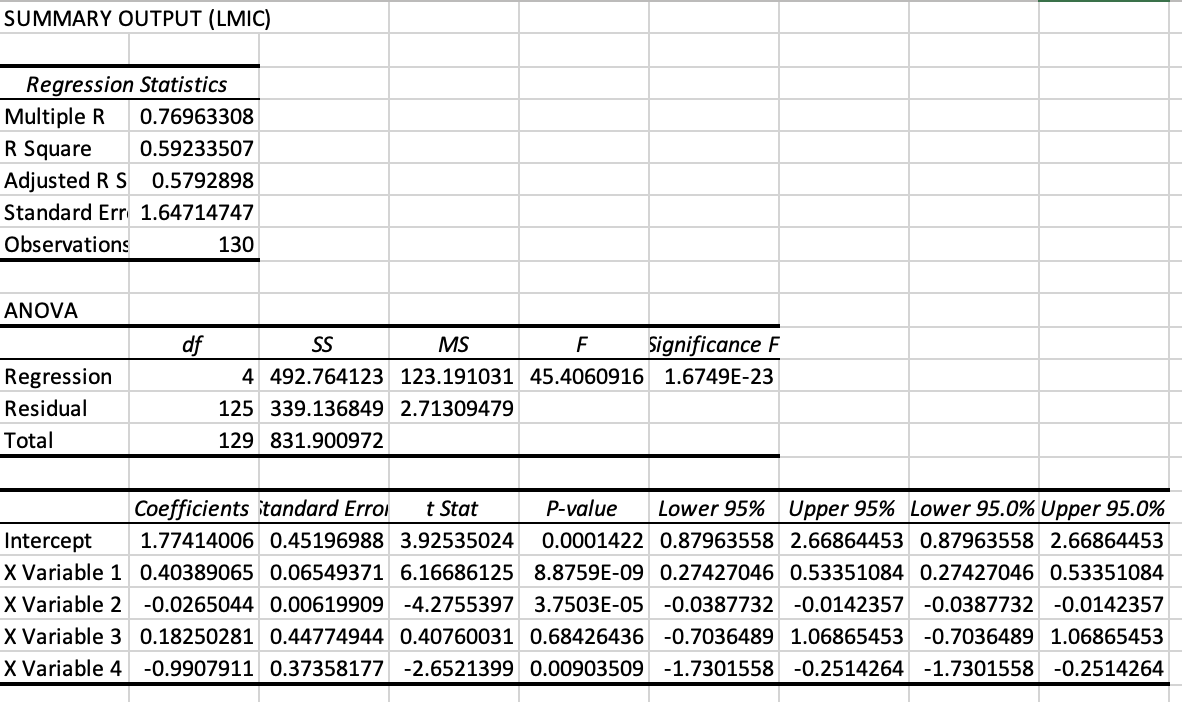
SUMMARY OUTPUT (HIC) \begin{tabular}{|l|r|r|r|r|r|} \hline \multicolumn{2}{|c|}{ Regression Statistics } & & & \\ \hline Multiple R & 0.58990972 & & & & \\ \hline R Square & 0.34799348 & & & & \\ \hline Adjusted R S & 0.29783914 & & & & \\ \hline Standard Err & 5.22305881 & & & & \\ \hline Observations & 57 & & & & \\ \hline & & & & & \\ \hline & & & & & \\ \hline ANOVA & & & & & \\ \hline & & SS & MS & & \\ \hline Regression & & 757.133303 & 189.283326 & 6.938451 & 0.00014881 \\ \hline Residual & 52 & 1418.57785 & 27.2803434 & & \\ \hline Total & 56 & 2175.71116 & & & \\ \hline \end{tabular} \begin{tabular}{|l|r|r|r|r|r|r|r|r|} \hline & Coefficients & tandard Erroi & \multicolumn{1}{|c|}{ S Stat } & \multicolumn{1}{|c|}{ P-value } & \multicolumn{1}{|c|}{ Lower 95\% } & \multicolumn{2}{|c|}{ Upper 95\% } & Lower 95.0\% Upper 95.0\% \\ \hline Intercept & 8.14227838 & 1.61612687 & 5.03814305 & 6.026E06 & 4.89928255 & 11.3852742 & 4.89928255 & 11.3852742 \\ \hline X Variable 1 & 0.07114274 & 0.03058344 & 2.32618502 & 0.02394144 & 0.00977258 & 0.13251291 & 0.00977258 & 0.13251291 \\ \hline X Variable 2 & -0.1914011 & 0.04799942 & -3.9875715 & 0.00020949 & -0.287719 & -0.0950832 & -0.287719 & -0.0950832 \\ \hline X Variable 3 & 3.3042092 & 1.49449394 & 2.21092178 & 0.03146321 & 0.30528771 & 6.30313068 & 0.30528771 & 6.30313068 \\ \hline X Variable 4 & -1.6344726 & 1.73141564 & -0.9440094 & 0.34953054 & -5.1088122 & 1.83986708 & -5.1088122 & 1.83986708 \\ \hline \end{tabular} SUMMARY OUTPUT (LMIC) \begin{tabular}{|l|r|r|r|r|r|} \hline \multicolumn{2}{|c|}{ Regression Statistics } & & & & \\ \hline Multiple R & 0.76963308 & & & & \\ \hline R Square & 0.59233507 & & & & \\ \hline Adjusted R S & 0.5792898 & & & & \\ \hline Standard Err & 1.64714747 & & & & \\ \hline Observations & 130 & & & & \\ \hline & & & & & \\ \hline ANOVA & & & & & \\ \hline & df & SS & MS & & \\ \hline Regression & 4 & 492.764123 & 123.191031 & 45.4060916 & 1.6749E23 \\ \hline Residual & 125 & 339.136849 & 2.71309479 & & \\ \hline Total & 129 & 831.900972 & & & \\ \hline \end{tabular} \begin{tabular}{|l|l|l|l|l|l|l|l|l|} \hline & Coefficients & tandard Errol & t Stat & P-value & Lower 95\% & Upper 95\% & Lower 95.0\% Upper 95.0\% \\ \hline Intercept & 1.77414006 & 0.45196988 & 3.92535024 & 0.0001422 & 0.87963558 & 2.66864453 & 0.87963558 & 2.66864453 \\ \hline X Variable 1 & 0.40389065 & 0.06549371 & 6.16686125 & 8.8759E09 & 0.27427046 & 0.53351084 & 0.27427046 & 0.53351084 \\ \hline X Variable 2 & -0.0265044 & 0.00619909 & -4.2755397 & 3.7503E05 & -0.0387732 & -0.0142357 & -0.0387732 & -0.0142357 \\ \hline X Variable 3 & 0.18250281 & 0.44774944 & 0.40760031 & 0.68426436 & -0.7036489 & 1.06865453 & -0.7036489 & 1.06865453 \\ \hline X Variable 4 & -0.9907911 & 0.37358177 & -2.6521399 & 0.00903509 & -1.7301558 & -0.2514264 & -1.7301558 & -0.2514264 \\ \hline \end{tabular}