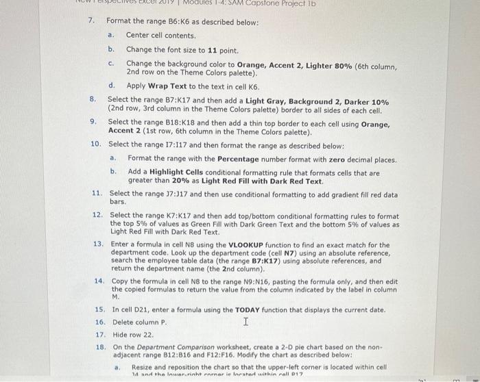
| Modules 1-4: SAM Capstone Project 1b Format the range B6:K6 as described below: 7. a. Center cell contents. b. Change the font size to 11 point. 8. 9. C. Change the background color to Orange, Accent 2, Lighter 80% (6th column, 2nd row on the Theme Colors palette). d. Apply Wrap Text to the text in cell K6. Select the range B7:K17 and then add a Light Gray, Background 2, Darker 10% (2nd row, 3rd column in the Theme Colors palette) border to all sides of each cell. Select the range B18:K18 and then add a thin top border to each cell using Orange, Accent 2 (1st row, 6th column in the Theme Colors palette). 10. Select the range 17:117 and then format the range as described below: a. b. Format the range with the Percentage number format with zero decimal places. Add a Highlight Cells conditional formatting rule that formats cells that are greater than 20% as Light Red Fill with Dark Red Text. 11. Select the range 37:317 and then use conditional formatting to add gradient fill red data bars. 12. Select the range K7:K17 and then add top/bottom conditional formatting rules to format the top 5% of values as Green Fill with Dark Green Text and the bottom 5% of values as Light Red Fill with Dark Red Text. 13. Enter a formula in cell N8 using the VLOOKUP function to find an exact match for the department code. Look up the department code (cell N7) using an absolute reference, search the employee table data (the range B7:K17) using absolute references, and return the department name (the 2nd column). 14. Copy the formula in cell NB to the range N9:N16, pasting the formula only, and then edit the copied formulas to return the value from the column indicated by the label in column M. 15. In cell D21, enter a formula using the TODAY function that displays the current date. 16. Delete column P. 17. Hide row 22. I 18. On the Department Comparison worksheet, create a 2-D pie chart based on the non- adjacent range B12:B16 and F12:F16. Modify the chart as described below: a. Resize and reposition the chart so that the upper-left corner is located within cell 14 and the Inwar.rinht earnar ie Inested within call 017