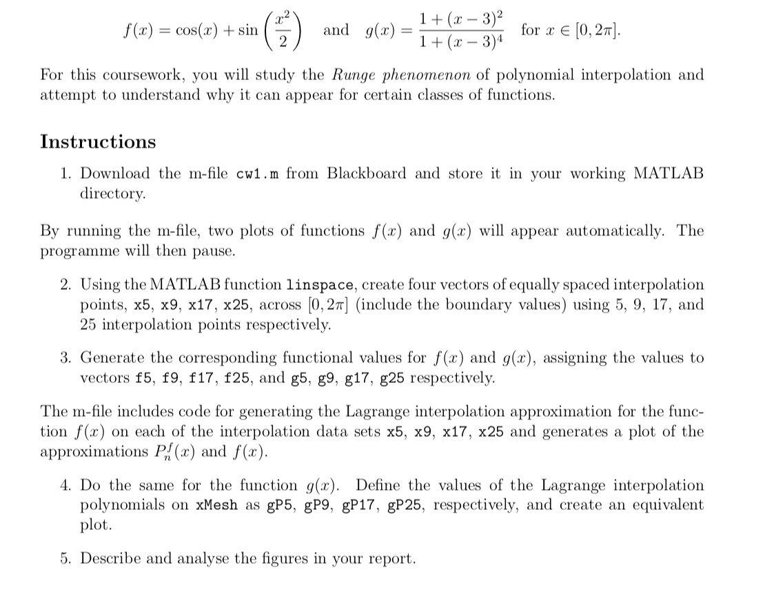
7- f(x) = cos(x) + sin and g(x) 1 + (x 3)2 1 + (x - 3) for x (0,21]. 2 For this coursework, you will study the Runge phenomenon of polynomial interpolation and attempt to understand why it can appear for certain classes of functions. Instructions 1. Download the m-file cw1.m from Blackboard and store it in your working MATLAB directory By running the m-file, two plots of functions f(x) and g(x) will appear automatically. The programme will then pause. 2. Using the MATLAB function linspace, create four vectors of equally spaced interpolation points, x5, x9, x17, x25, across [0, 27] (include the boundary values) using 5, 9, 17, and 25 interpolation points respectively. 3. Generate the corresponding functional values for f(x) and g(x), assigning the values to vectors f5, f9, f17, f25, and g5, g9, g17, g25 respectively. The m-file includes code for generating the Lagrange interpolation approximation for the func- tion f(x) on each of the interpolation data sets x5, x9, x17, x25 and generates a plot of the approximations P.:(x) and f(x). 4. Do the same for the function g(x). Define the values of the Lagrange interpolation polynomials on xMesh as gP5, gP9, gP17, gP25, respectively, and create an equivalent plot. 5. Describe and analyse the figures in your report. 7- f(x) = cos(x) + sin and g(x) 1 + (x 3)2 1 + (x - 3) for x (0,21]. 2 For this coursework, you will study the Runge phenomenon of polynomial interpolation and attempt to understand why it can appear for certain classes of functions. Instructions 1. Download the m-file cw1.m from Blackboard and store it in your working MATLAB directory By running the m-file, two plots of functions f(x) and g(x) will appear automatically. The programme will then pause. 2. Using the MATLAB function linspace, create four vectors of equally spaced interpolation points, x5, x9, x17, x25, across [0, 27] (include the boundary values) using 5, 9, 17, and 25 interpolation points respectively. 3. Generate the corresponding functional values for f(x) and g(x), assigning the values to vectors f5, f9, f17, f25, and g5, g9, g17, g25 respectively. The m-file includes code for generating the Lagrange interpolation approximation for the func- tion f(x) on each of the interpolation data sets x5, x9, x17, x25 and generates a plot of the approximations P.:(x) and f(x). 4. Do the same for the function g(x). Define the values of the Lagrange interpolation polynomials on xMesh as gP5, gP9, gP17, gP25, respectively, and create an equivalent plot. 5. Describe and analyse the figures in your report