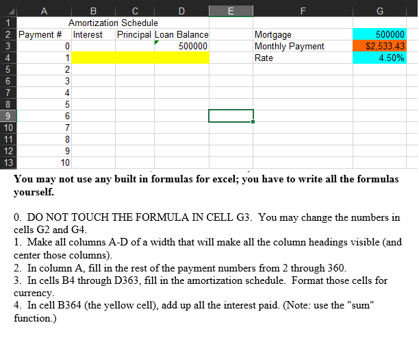
A B D E F G Amortization Schedule 2 Payment # Interest Principal Loan Balance Mortgage 500000 3 0 500000 Monthly Payment $2,533.43 4 1 Rate 4.50% 5 2 6 3 7 4 8 5 9 6 10 7 11 8 12 9 13 10 You may not use any built in formulas for excel; you have to write all the formulas yourself. 0. DO NOT TOUCH THE FORMULA IN CELL G3. You may change the numbers in cells G2 and G4. 1. Make all columns A-D of a width that will make all the column headings visible and center those columns). 2. In column A, fill in the rest of the payment numbers from 2 through 360. 3. In cells B4 through D363, fill in the amortization schedule. Format those cells for currency. 4. In cell B364 (the yellow cell), add up all the interest paid. (Note: use the "sum" function.)