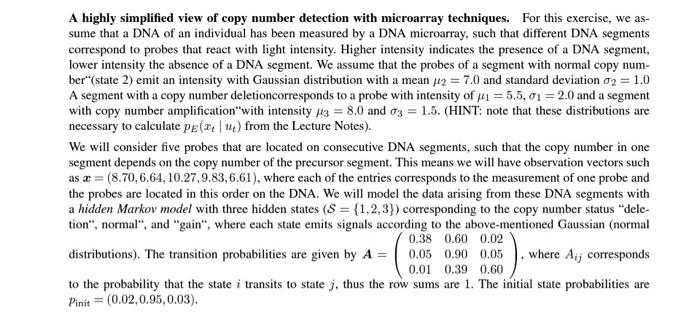
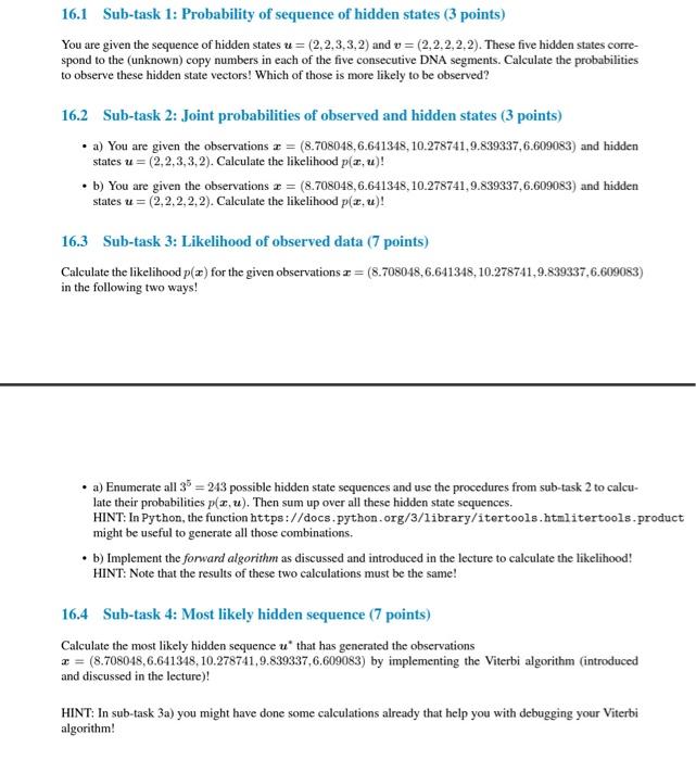
A highly simplified view of copy number detection with microarray techniques. For this exercise, we assume that a DNA of an individual has been measured by a DNA microarray, such that different DNA segments correspond to probes that react with light intensity. Higher intensity indicates the presence of a DNA segment, lower intensity the absence of a DNA segment. We assume that the probes of a segment with normal copy number"(state 2) emit an intensity with Gaussian distribution with a mean 2=7.0 and standard deviation 2=1.0 A segment with a copy number deletioncorresponds to a probe with intensity of 1=5.5,1=2.0 and a segment with copy number amplification "with intensity 3=8.0 and 3=1.5. (HINT: note that these distributions are necessary to calculate pE(xtut) from the Lecture Notes). We will consider five probes that are located on consecutive DNA segments, such that the copy number in one segment depends on the copy number of the precursor segment. This means we will have observation vectors such as x=(8.70,6.64,10.27,9.83,6.61), where each of the entries corresponds to the measurement of one probe and the probes are located in this order on the DNA. We will model the data arising from these DNA segments with a hidden Markov model with three hidden states (S={1,2,3}) corresponding to the copy number status "deletion", normal", and "gain", where each state emits signals according to the above-mentioned Gaussian (normal distributions). The transition probabilities are given by A=0.380.050.010.600.900.390.020.050.60, where Aij corresponds to the probability that the state i transits to state j, thus the row sums are 1 . The initial state probabilities are pinit=(0.02,0.95,0.03) You are given the sequence of hidden states u=(2,2,3,3,2) and v=(2,2,2,2,2). These five hidden states correspond to the (unknown) copy numbers in each of the five consecutive DNA segments. Calculate the probabilities to observe these hidden state vectors! Which of those is more likely to be observed? 16.2 Sub-task 2: Joint probabilities of observed and hidden states (3 points) - a) You are given the observations x=(8.708048,6.641348,10.278741,9.839337,6.609083) and hidden states u=(2,2,3,3,2). Calculate the likelihood p(x,u)! - b) You are given the observations x=(8.708048,6.641348,10.278741,9.839337,6.609083) and hidden states u=(2,2,2,2,2). Calculate the likelihood p(x,u)! 16.3 Sub-task 3: Likelihood of observed data (7 points) Calculate the likelihood p(x) for the given observations x=(8.708048,6.641348,10.278741,9.839337,6.609083) in the following two ways! - a) Enumerate all 35=243 possible hidden state sequences and use the procedures from sub-task 2 to calculate their probabilities p(x,u). Then sum up over all these hidden state sequences. HINT: In Python, the function https://docs,python.org/3/1ibrary/itertools.htm1itertools,product might be useful to generate all those combinations. - b) Implement the forward algorithm as discussed and introduced in the lecture to calculate the likelihood! HINT: Note that the results of these two calculations must be the same! 16.4 Sub-task 4: Most likely hidden sequence (7 points) Calculate the most likely hidden sequence u that has generated the observations x=(8.708048,6.641348,10.278741,9.839337,6.609083) by implementing the Viterbi algorithm (introduced and discussed in the lecture)! HINT: In sub-task 3a) you might have done some calculations already that help you with debugging your Viterbi algorithm