A linear function was used to compute forecasts for a time series with seasonality. These are the results of the residual analysis:

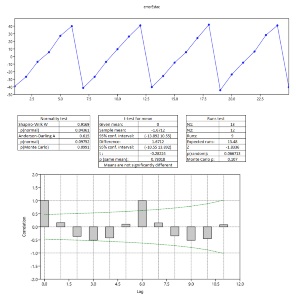
Mark all the statements that are true:

a. Evidence indicates that the residuals are independent

b. The residuals are centered at mean zero.

c. It is very unlikely that the residuals come from a Normal population

d. The graph of the autocorrelation function does not show significant correlations

e. The residuals present homoscedasticity

emorfstac \begin{tabular}{|c|r|} \hline \multicolumn{2}{|c|}{ Normality test } \\ \hline Shapiro-Wilk W & 0.9169 \\ \hline p (normal) & 0.04361 \\ \hline Anderson-Darling A & 0.615 \\ \hline p (normal) & 0.09752 \\ \hline p (Monte Carlo) & 0.0991 \\ \hline \end{tabular} \begin{tabular}{|l|c|} \hline \multicolumn{2}{|c|}{ t-test for mean } \\ \hline Given mean: & 0 \\ \hline Sample mean: & 1.6712 \\ \hline 95% conf. interval: & (13.89210.55) \\ \hline Difference: & 1.6712 \\ \hline 95% conf. interval: & (10.5513.892) \\ \hlinet: & 0.28224 \\ \hlinep (same mean): & 0.78018 \\ \hline \multicolumn{2}{|c|}{ Means are not significantly different } \\ \hline \end{tabular} \begin{tabular}{|l|c|} \hline \multicolumn{2}{|c|}{ Runs test } \\ \hline N1: & 13 \\ \hline N2: & 12 \\ \hline Runs: & 9 \\ \hline Expected runs: & 13.48 \\ \hlineZ & 1.8336 \\ \hline p (random): & 0.066713 \\ \hline Monte Carlo p: & 0.107 \\ \hline \end{tabular}