Question: A microcomputer manufacturer has developed a regression model relating his sales (Y in $10,000s) with three independent variables. The three independent variables are price per

A microcomputer manufacturer has developed a regression model relating his sales (Y in $10,000s) with three independent variables. The three independent variables are price per unit (Price in $100s), advertising (ADV in $1,000s) and the number of product lines (Lines). Part of the regression results is shown below.

in $10,000s) with three independent variables. The three independent variables are price

per unit (Price in $100s), advertising (ADV in $1,000s) and the number

of product lines (Lines). Part of the regression results is shown below.

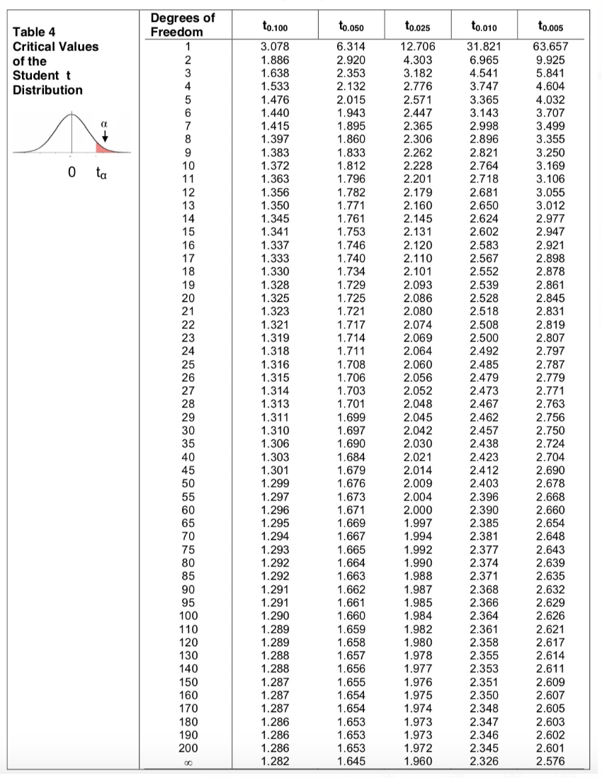
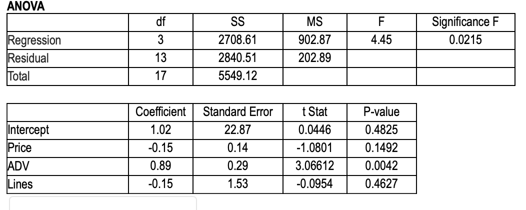
Degrees of Table 4 Freedom to. 100 to.050 to.025 to.010 to.005 Critical Values 3.078 6.314 12.706 31.821 63.657 of the 1.886 2.920 4.303 6.965 9.925 Student t 1.638 2.353 3.182 4.541 5.841 Distribution 1.533 2. 132 NODAWN 2.776 3.747 4.604 1.476 2.015 2.571 3.365 4.032 1.440 1.943 2.447 3.143 3.707 1.415 1.895 + R 2.365 2.998 3.499 8 1.397 1.860 2.306 2.896 3.355 9 1.383 1.833 2.262 2.821 3.250 0 ta 10 1.372 1.812 2.228 2.764 3.169 11 1.363 1.796 2.201 2.718 3.106 12 1.356 1.782 2.179 2.681 13 3.055 1.350 1.771 2.160 2.650 14 3.012 1.345 1.761 15 2.145 2.624 2.977 1.341 1.753 2.131 2.602 2.947 16 1.337 1.746 2.120 2.583 2.921 17 1.333 1.740 2.110 2.567 2.898 18 1.330 1.734 2.101 2.552 2.878 19 1.328 1.729 2.093 2.539 2.861 20 1.325 1.725 2.086 2.528 2.845 21 1.323 1.721 2.080 2.518 22 2.831 1.321 1.717 2.074 2.508 23 2.819 1.319 1.714 2.069 2.500 24 2.807 1.318 1.711 2.064 2.492 2.797 25 1.316 1.708 2.060 2.485 2.787 26 1.315 1.706 2.056 2.479 27 2.779 1.314 1.703 2.052 2.473 28 2.771 1.313 1.701 2.048 2.467 2.763 29 1.311 1.699 2.045 2.462 2.756 30 1.310 1.697 2.042 2.457 35 2.750 1.306 1.690 2.030 2.438 2.724 40 1.303 1.684 2.021 2.423 45 2.704 1.301 1.679 2.014 2.412 2.690 50 1.299 1.676 2.009 2.403 2.678 55 1.297 1.673 2.004 2.396 60 2.668 1.296 1.671 2.000 2.390 2.660 65 1.295 1.669 1.997 2.385 2.654 70 1.294 1.667 1.994 2.381 2.648 75 1.293 1.665 1.992 2.377 2.643 80 1.292 1.664 1.990 2.374 85 2.639 1.292 1.663 1.988 2.371 2.635 90 1.291 1.662 1.987 2.368 2.632 95 1.291 1.661 1.985 2.366 2.629 100 1.290 1.660 1.984 2.364 2.626 110 1.289 1.659 1.982 2.361 2.621 120 1.289 1.658 1.980 2.358 130 2.617 1.288 1.657 1.978 2.355 2.614 140 1.288 1.656 1.977 2.353 2.611 150 1.287 1.655 1.976 2.351 2.609 160 1.287 1.654 1.975 2.350 2.607 170 1.287 1.654 1.974 2.348 2.605 180 1.286 1.653 1.973 2.347 2.603 190 1.286 1.653 1.973 2.346 2.602 200 1.286 1.653 1.972 2.345 2.601 00 1.282 1.645 1.960 2.326 2.576\f\fANOVA of SS MS F Significance F Regression 2708.61 902.87 4.45 0.0215 Residual 13 2840.51 202.89 Total 17 5549.12 Coefficient Standard Error t Stat P-value Intercept 1.02 22.87 0.0446 0.4825 Price -0.15 0.14 -1.0801 0. 1492 ADV 0.89 0.29 3.06612 0.0042 Lines -0.15 1.53 -0.0954 0.4627

Step by Step Solution

There are 3 Steps involved in it

1 Expert Approved Answer

Step: 1 Unlock blur-text-image

Question Has Been Solved by an Expert!

Get step-by-step solutions from verified subject matter experts

Step: 2 Unlock

Step: 3 Unlock

Students Have Also Explored These Related Mathematics Questions!

26. A microcomputer manufacturer has developed a regression model relating his sales (Y in $10,000s) with three independent variables. The three independent variables are price per unit (Price in...

please help D Question 37 1 pts Problem 4. A computer manufacturer has developed a regression model relating Sales (y) with four independent variables. The four independent variables are Price (in...

Problem 4. A computer manufacturer has developed a regression model relating Sales ( y ) with four independent variables. The four independent variables are Price (in dollars), Competitor's Price (in...

Please provide all work included in the answer. Thank you. ._ [15 points]. A microcomputer manufacturer has developed a regression model relating his sales (Y in $10,000s) with three independent...

1.Amicrocomputermanufacturer has developed a regression model relating his sales (y in $10,000s) with three independent variables. The three independent variables are price per unit (Price in $100s),...

The Natural Drink Company has developed a regression model relating their sales (Y in 10,0005), with three independent variables. The three independent variables are price per unit (X1 in pounds),...

Question 1A A real estate research firm has developed a regression model relating list price (Y in $1,000) with two independent variables. The two independent variables are number of bedrooms and...

P&G Facelle division a. Highlight potential decisions required in the case & which factors should P&G consider before making thesedecisions b. How are their own brands performing? Analyze in detail...

Stock Prices Business Statistics-Semester Project Introduction: The stock market is a very powerful investing tool and very difficult to understand. The stock market is simply a place where stocks...

summarize and raise outstanding issues about managerial accounting in the article Accounting Information for Product Costing - Case Study Suzana Keglevi Kozjak, Tanja estanj-Peri Faculty of...

Let (a) Find an orthogonal basis for comg A. (b) Find an orthogonal basis for ker A. (c) If you combine your bases from part (a) and (b), do you get an orthogonal basis of R4? Why or why not? 24-2...

What price do farmers get for their strawberry crops? In the third week of April, a random sample of 43 farms gave a sample mean of $66.00 per 10 pounds of strawberries. Assume that o is known to be...

Work with a partner or in a small group to discuss this question. What is the quickest method to use to work out the answer to 6 5/8 3 1/2?

Over the next 90 days, economists forecast that the pound may strengthen relative to the dollar by as much as 12%, or it may weaken by as much as 9%. The possible values for the rate of change of the...