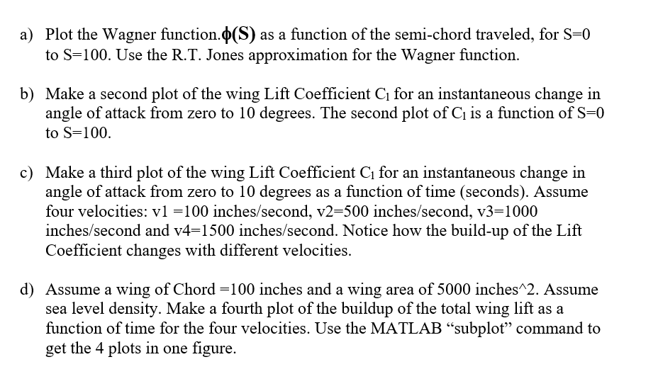
a$)$ Plot the Wagner function. $\backslash (\backslash$boldsymbol$\{\backslash$phi$\}\backslash$mathbf$\{($ S $)\}\backslash )$ as a function of the semi$-$chord traveled, for $\backslash (\backslash$mathrm$\{$S$\}=0\backslash )$ to $\backslash ($ S$=100\backslash ).$ Use the R$.$T$.$ Jones approximation for the Wagner function.

b$)$ Make a second plot of the wing Lift Coefficient $\backslash (\backslash$mathrm$\{$C$\}\_\{1\}\backslash )$ for an instantaneous change in angle of attack from zero to $10$ degrees. The second plot of $\backslash ($ C$\_\{1\}\backslash )$ is a function of $\backslash ($ S$=0\backslash )$ to $\backslash ($ S$=100\backslash ).$

c$)$ Make a third plot of the wing Lift Coefficient $\backslash (\backslash$mathrm$\{$C$\}\_\{1\}\backslash )$ for an instantaneous change in angle of attack from zero to $10$ degrees as a function of time $($seconds$).$ Assume four velocities: $\backslash (\backslash$mathrm$\{$v$\}1=100\backslash )$ inches$/$second$,\backslash (\backslash$mathrm$\{$v$\}2=500\backslash )$ inches$/$second$,\backslash (\backslash$mathrm$\{$v$\}3=1000\backslash )$ inches$/$second and v$4=1500$ inches$/$second$.$ Notice how the build$-$up of the Lift Coefficient changes with different velocities.

d$)$ Assume a wing of Chord $=100$ inches and a wing area of $5000$ inches$^2.$ Assume sea level density. Make a fourth plot of the buildup of the total wing lift as a function of time for the four velocities. Use the MATLAB "subplot" command to get the $4$ plots in one figure.