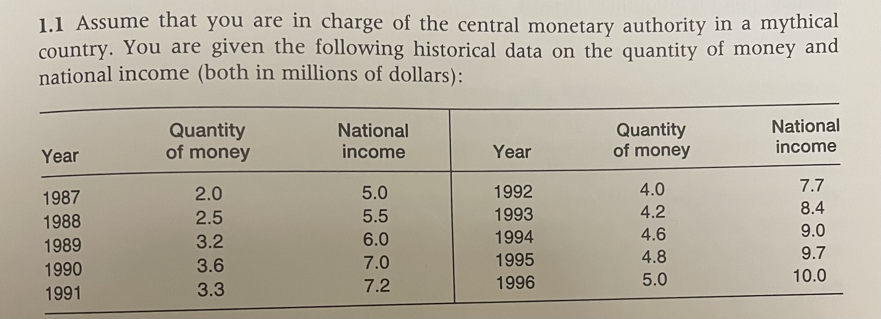
(a) Plot these points on a scatter diagram. Then estimate the regression of national income Y on the quantity of money X and plot the line on the scatter diagram. (b) How do you interpret the intercept and slope of the regression line? () If you had sole control over the money supply and wished to achieve a level of national income of 12.0 in 1997, at what level would you set the money supply? Explain. 1.2 Calculate the regression of income on grade-point average in the example described in this chapter and compare it with the regression of grade-point average on income. Why are the two results different? 1.3 (a) Assume thatleast-squares estimates are obtained for the relationship = a + bX. After the work is completed, it is decided to multiply the units of the X variable by a factor of 10. What will happen to the resulting least-squares slope and intercept? (b) Generalize the result of part (a) by evaluating the effects on the regression of changing the units of X and Y in the following manner: Y*=C1+C2Y X*=dl+d2X What can you conclude? 1.4 What happens to the least-squares intercept and the slope estimate when all observations on the independent variable are identical? Can you explain intuitively why this occurs? 1.1 Assume that you are in charge of the central monetary authority in a mythical country. You are given the following historical data on the quantity of money and national income (both in millions of dollars) : Quantity National Quantity National Year of money income Year of money income 1987 2.0 5.0 1992 4.0 7.7 1988 2.5 5.5 1993 4.2 8.4 1989 3.2 6.0 1994 4.6 9.0 1990 3.6 7.0 1995 4.8 9.7 1996 10.0 1991 3.3 7.2 5.0