a$.$ Start Excel, open IL$\_$EX$\_8-4.$xlsx from the location where you store your Data Files, then save it as IL$\_$EX$\_8\_$Accommodations.

b$.$ Create a PivotTable on a new worksheet named PivotTable that sums the revenue amount for each region across the rows and each purpose down the columns. Add the quarter field as an inner row label. Use FIGURE $8-27$ as a guide.

c$.$ Widen column $C$ of the PivotTable if necessary to fully display the grand total value for that column.

FIGURE $8-27$

d$.$ Group the first two quarters $($Hint: Select the first two quarter cells in any region, then click the Group Selection button in the Group group on the PivotTable Analyze tab.$)$

e$.$ Rename the Group$1$ label First Half. $($Hint: Enter the new name in any cell with the Group$1$ label.$)$

f$.$ Group the third and fourth quarters, then name this new group Last Half.

g$.$ Collapse both the First Half and Last Half groups.

h$.$ Turn off the grand totals for the Columns. $($Hint: Click the Grand Totals button in the Layout group on the PivotTable Tools Design tab, then click On for Rows Only.$)$

i$.$ Format the revenue values using the Currency format with the $ symbol and no decimal places.

j$.$ On the Revenue worksheet, change the North America Quarter $1$ Business Revenue value in cell D$2$ to $s Update the PivotTable to reflect this increase in revenue.

k$.$ Create a stacked column PivotChart report for the revenue data for all three regions. $($Hint: Choose Stacked Column Chart type in the dialog box.$)$

Move the PivotChart to a new sheet, and name the chart sheet PivotChart.

m$.$ Apply a quick layout of Layout $4$ to the PivotChart.

n$.$ Use the Region field button at the bottom of the PivotChart to filter the chart to display only Euro$]$ America properties.

o$.$ Add a Quarter $2$ slicer to the PivotTable. Use the slicer to display the revenue for the first half of the

p$.$ Check the PivotChart to be sure it displays only the filtered data.

q$.$ On the PivotTable sheet, resize the slicer to display the button in two columns that are each ${0\mathrm{.}5}^{\text{'}\text{'}}h$ width. $($Hint: Use the Buttons group on the Slicer Tools Options tab.$)$

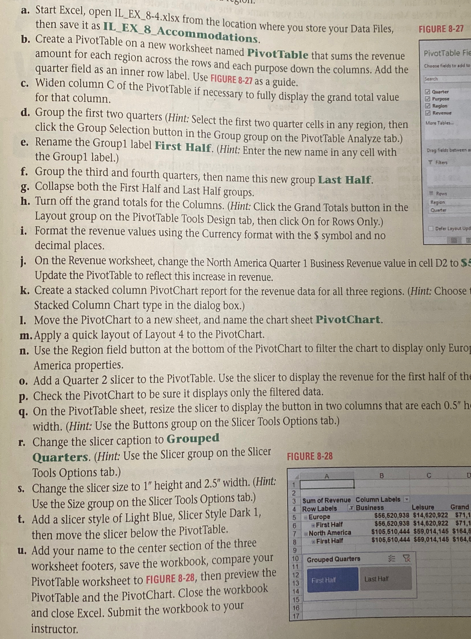
r$.$ Change the slicer caption to Grouped

Quarters. $($Hint: Use the Slicer group on the Slicer Tools Options tab.$)$

s$.$ Change the slicer size to $1^{\text{'}\text{'}}$ height and ${2\mathrm{.}5}^{\text{'}\text{'}}$ width. $($Hint: Use the Size group on the Slicer Tools Options tab.$)$

t$.$ Add a slicer style of Light Blue, Slicer Style Dark $1,$ then move the slicer below the PivotTable.

u$.$ Add your name to the center section of the three worksheet footers, save the workbook, compare your PivotTable worksheet to FIGURE $8-28,$ then preview the PivotTable and the PivotChart. Close the workbook and close Excel. Submit the workbook to your instructor.

FIGURE $8-28$