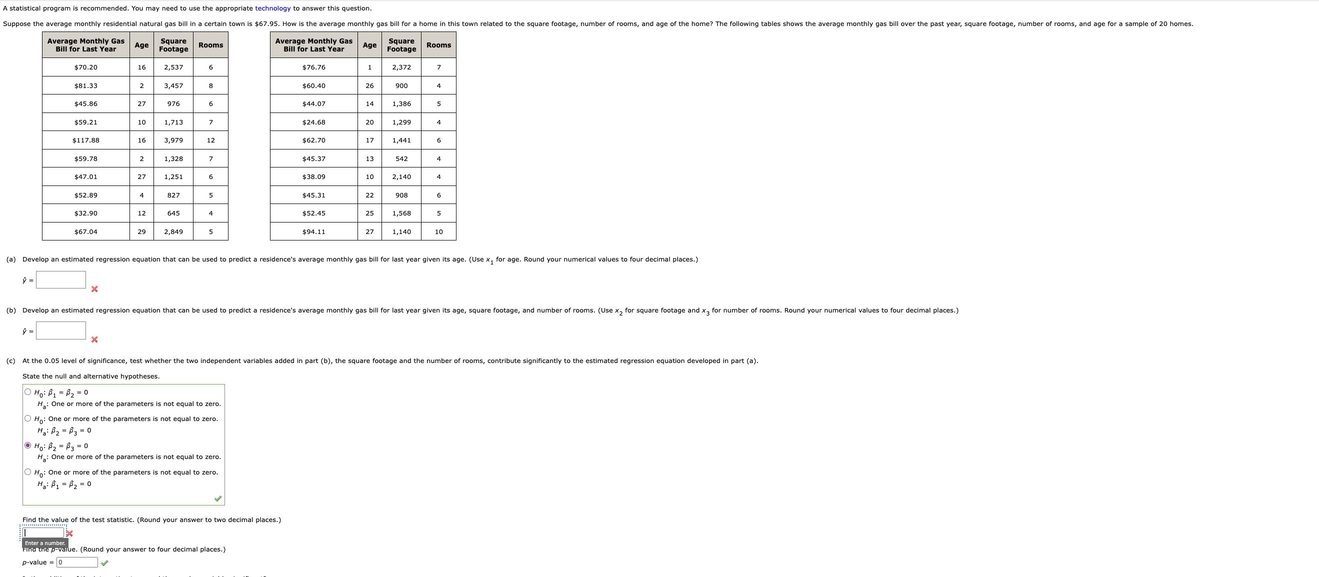
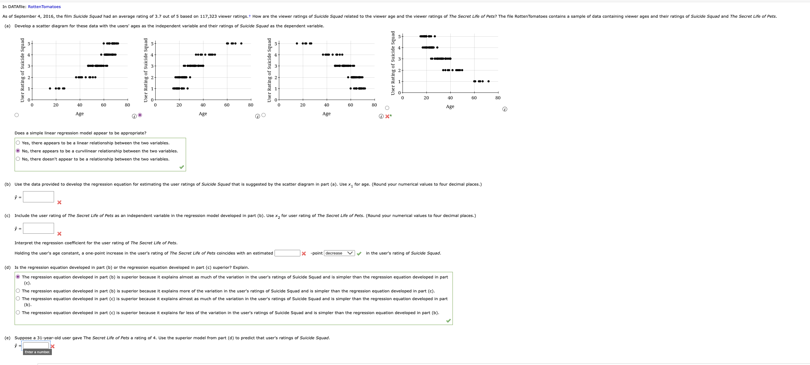
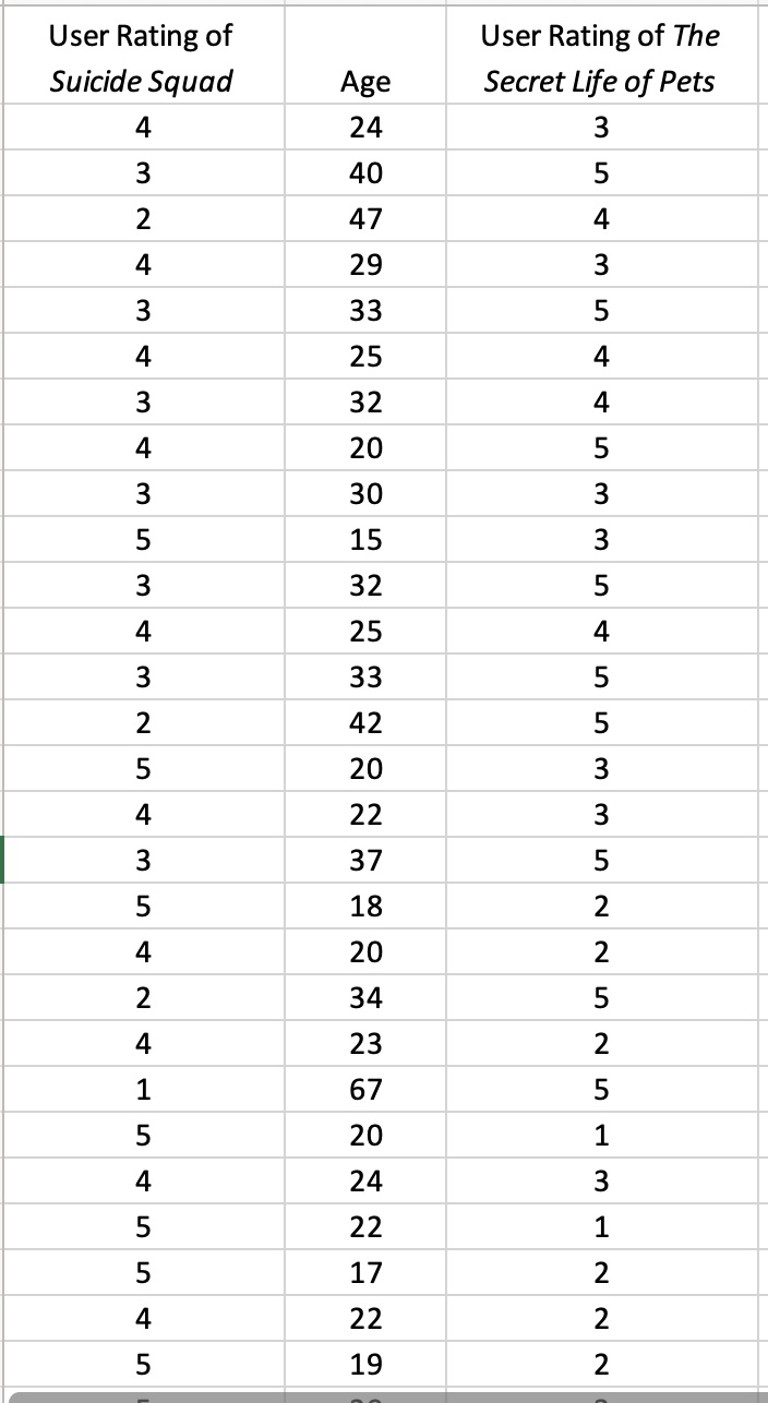
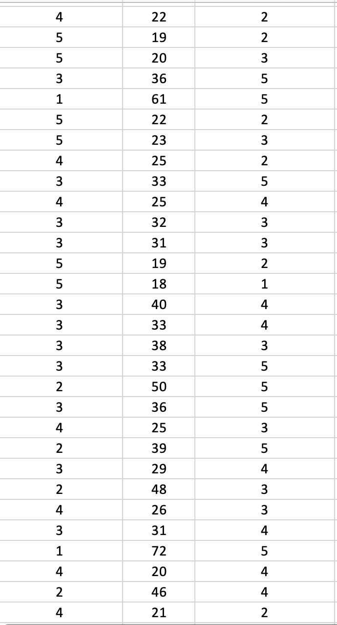
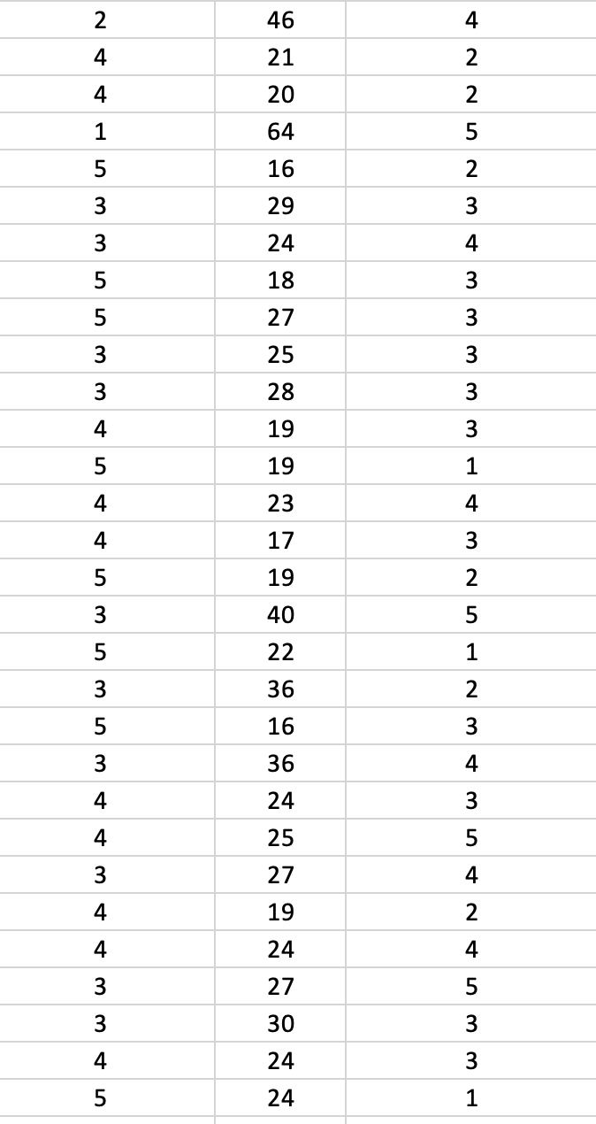
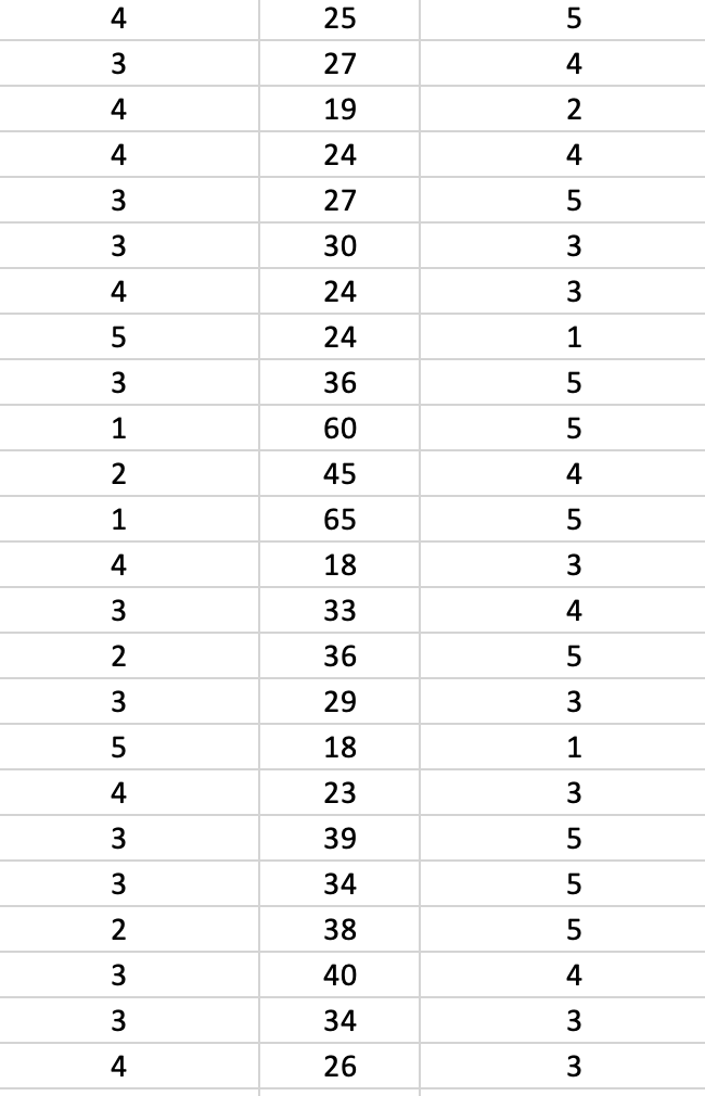
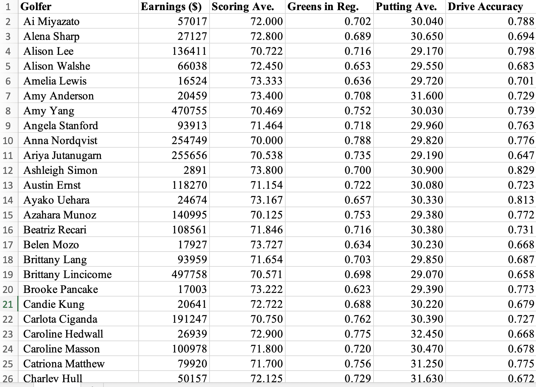
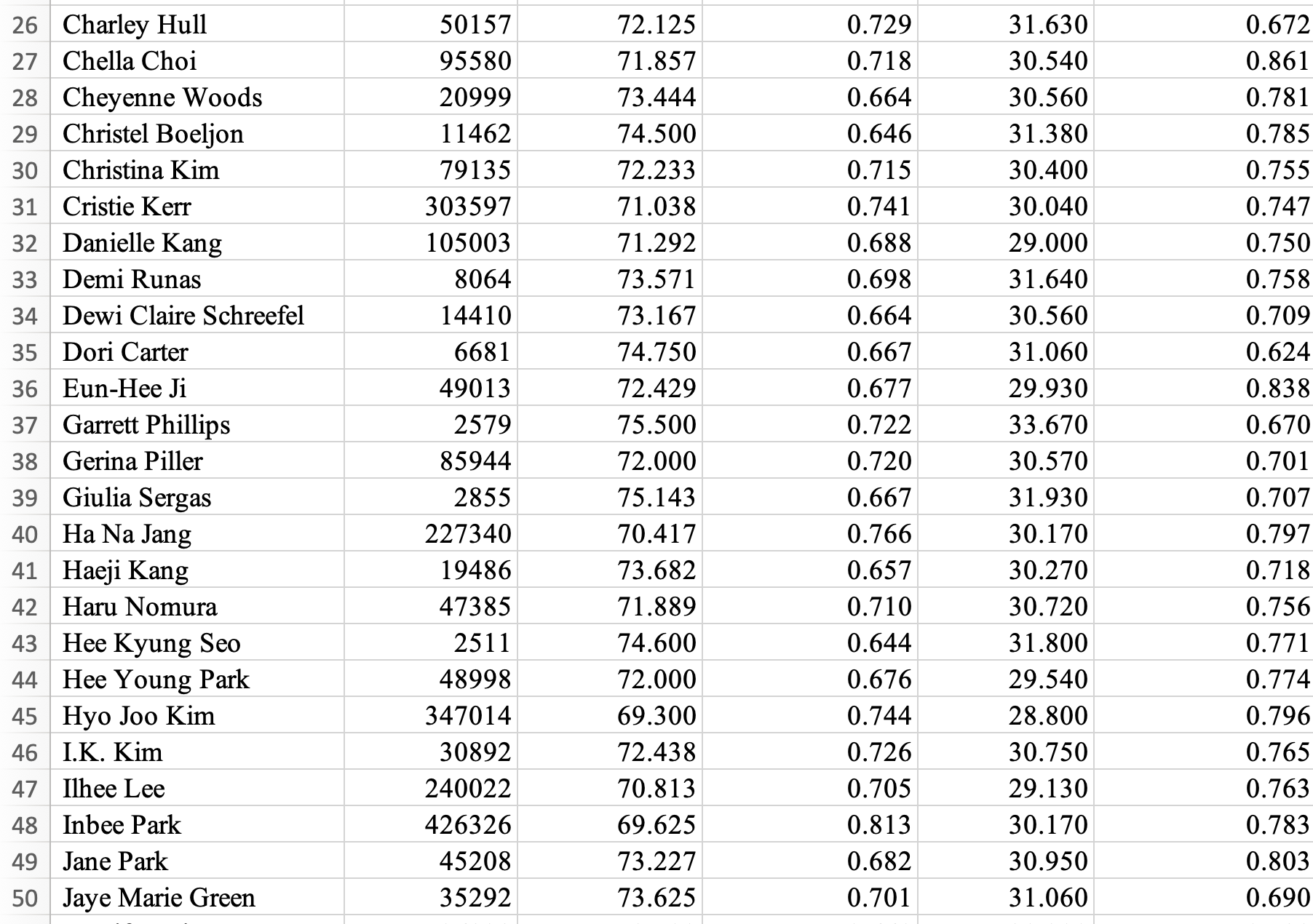
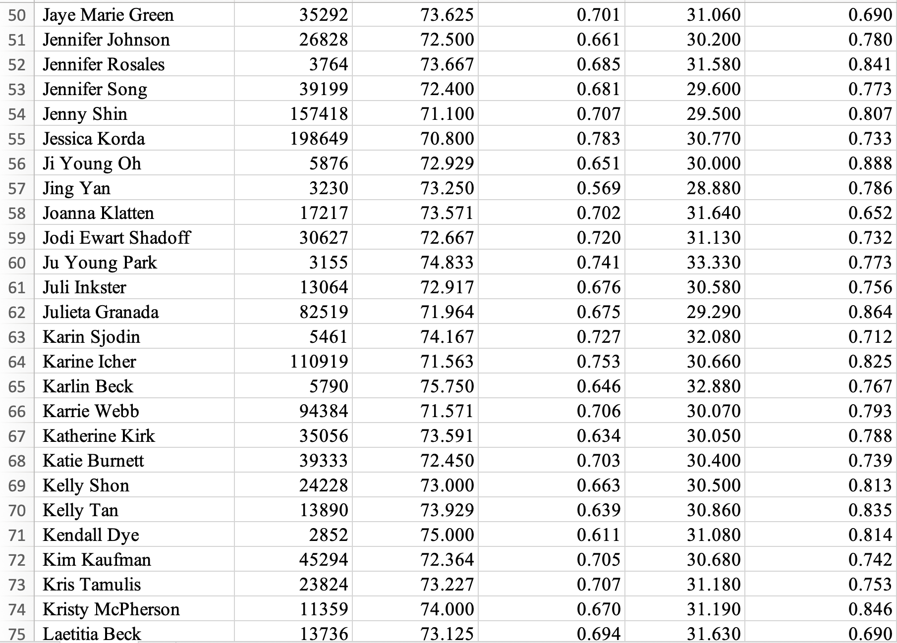
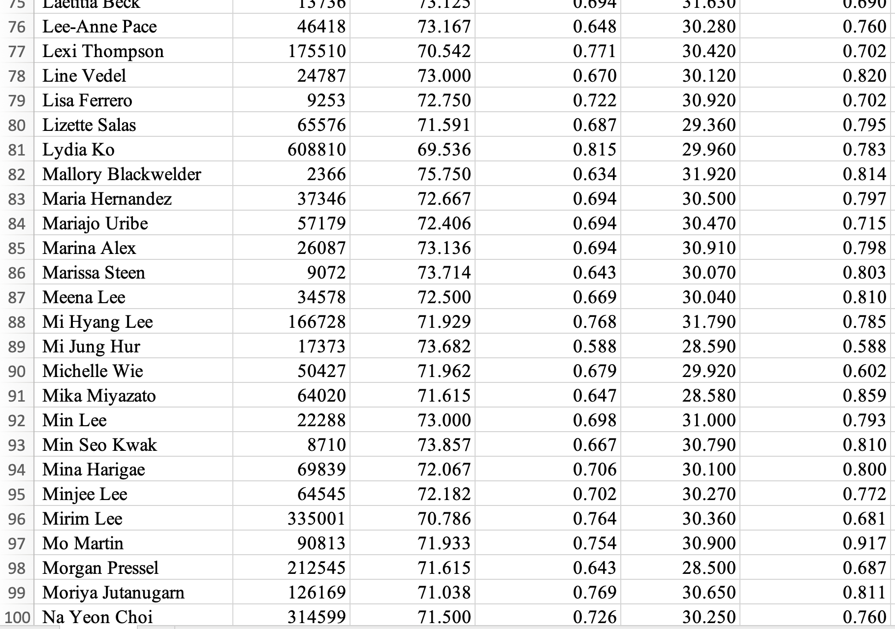
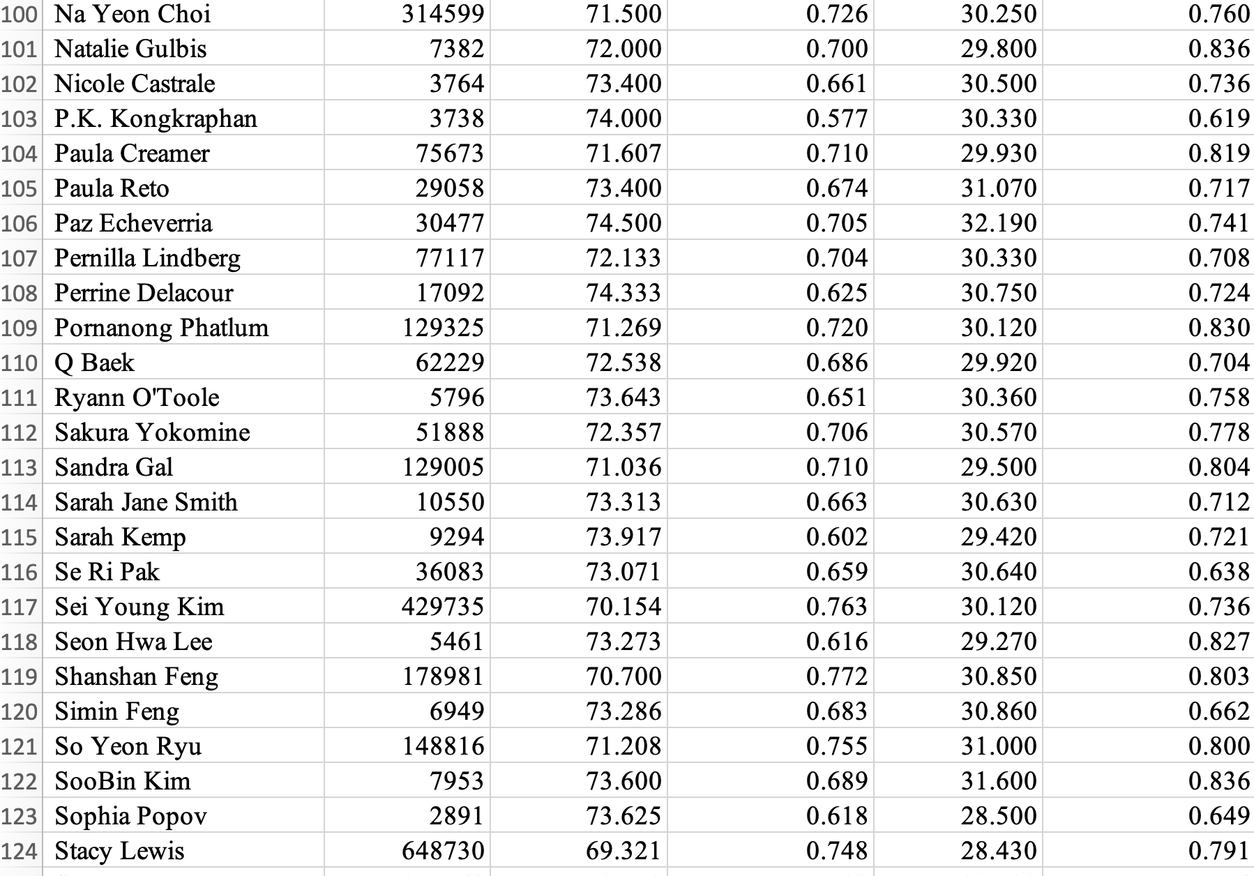
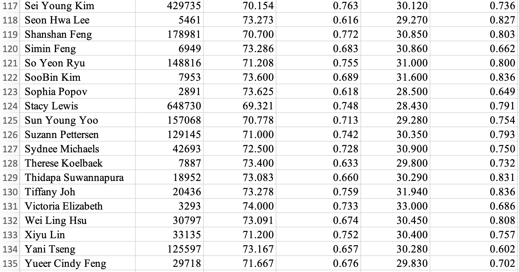
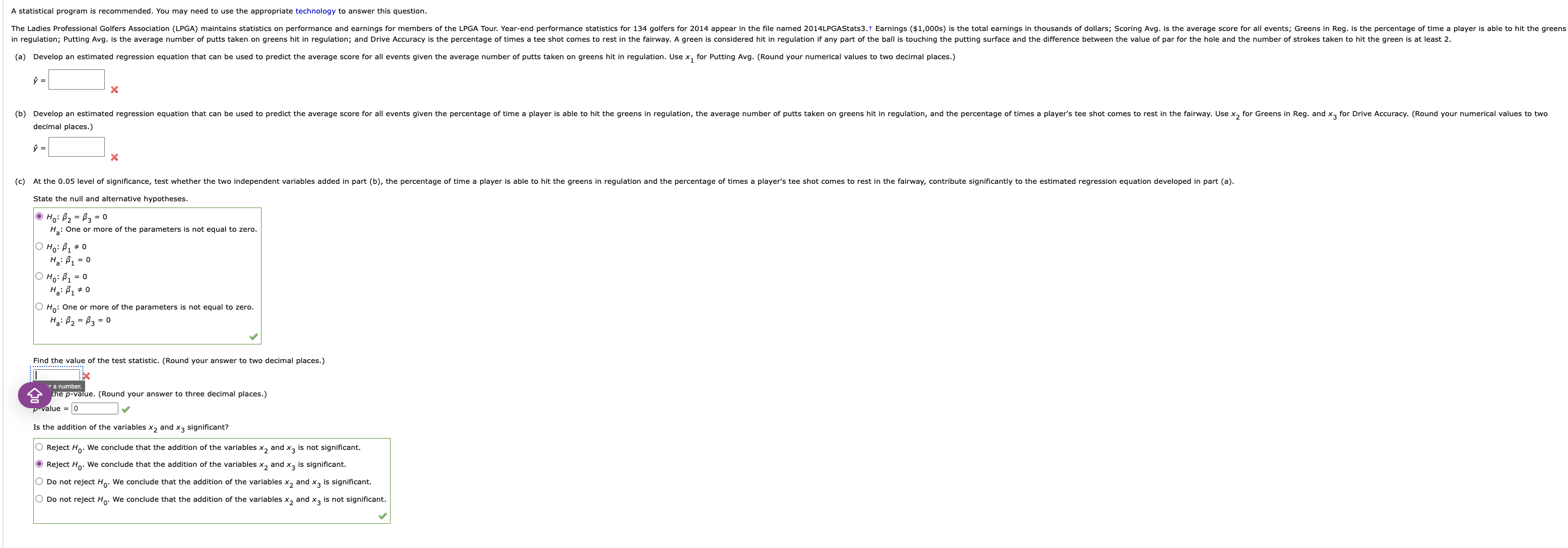
A statistical program is recommended. You may need to use the appropriate technology to answer this question. Suppose the average monthly residential natural gas bill in a certain town is $67.95. How is the average monthly gas bill for a home in this town related to the square footage, number of rooms, and age of the home? The following tables shows the average monthly gas bill over the past year, square footage, number of rooms, and age for a sample of 20 homes. Average Monthly Gas Bill for Last Year Age Square Footage Rooms Average Monthly Gas Square Bill for Last Year Age Footage Rooms $70.20 16 2,537 6 $76.76 2,372 $81.33 2 3,457 60.40 26 900 $45.86 27 976 44.07 14 1,386 $59.21 10 1,713 $24.68 20 1,299 $117.88 16 3,979 12 $62.70 17 1,441 $59.78 1,328 $45.37 13 54 $47.01 27 1,251 6 $38.09 10 2,140 $52.89 827 5 $45.31 22 908 6 $32.90 12 645 4 $52.45 25 1,568 5 $67.04 29 2,849 $94.11 27 1,140 10 (a) Develop an estimated regression equation that can be used to predict a residence's average monthly gas bill for last year given its age. (Use x, for age. Round your numerical values to four decimal places.) D = (b) Develop an estimated regression equation that can be used to predict a residence's average monthly gas bill for last year given its age, square footage, and number of rooms. (Use x2 for square footage and X3 for number of rooms. Round your numerical values to four decimal places.) y = (c) At the 0.05 level of significance, test whether the two independent variables added in part (b), the square footage and the number of rooms, contribute significantly to the estimated regression equation developed in part (a). State the null and alternative hypotheses O Ho: B1 = $2 = 0 Ha: One or more of the parameters is not equal to zero. O Ho: One or more of the parameters is not equal to zero. Ha: B2 = B3 = 0 O Ho: B2 = B3 = 0 Ha: One or more of the parameters is not equal to zero. O Ho: One or more of the parameters is not equal to zero. Ha: B1 = $2 = 0 Find the value of the test statistic. (Round your answer to two decimal places.) Enter a number. ina the p-value. (Round your answer to four decimal places.) P-value = 0In DATAfile: Rotten Tomatoes As of September 4, 2016, the film Suicide Squad had an average rating of 3.7 out of 5 based on 117,323 viewer ratings. How are the viewer ratings of Suicide Squad related to the viewer age and the viewer ratings of The Secret Life of Pets? The file Rotten Tomatoes contains a sample of data containing viewer ages and their ratings of Suicide Squad and The Secret Life of Pets. (a) Develop a scatter diagram for these data with the users' ages as the independent variable and their ratings of Suicide Squad as the dependent variable . 0. 57 . .. 4 4+ omm . ... User Rating of Suicide Squad 3+ User Rating of Suicide Squad User Rating of Suicide Squad User Rating of Suicide Squad N N 2 . . . . .. . O of 20 10 60 80 20 40 60 30 20 40 60 80 0 20 10 60 80 Age Age Age Age Does a simple linear regression model appear to be appropriate? O Yes, there appears to be a linear relationship between the two variables. No, there appears to be a curvilinear relationship between the two variables. O No, there doesn't appear to be a relationship between the two variables. (b) Use the data provided to develop the regression equation for estimating the user ratings of Suicide Squad that is suggested by the scatter diagram in part (a). Use x, for age. (Round your numerical values to four decimal places.) y = (c) Include the user rating of The Secret Life of Pets as an independent variable in the regression model developed in part (b). Use x2 for user rating of The Secret Life of Pets. (Round your numerical values to four decimal places.) y = x Interpret the regression coefficient for the user rating of The Secret Life of Pets. Holding the user's age constant, a one-point increase in the user's rating of The Secret Life of Pets coincides with an estimated X -point decrease V . in the user's rating of Suicide Squad. (d) Is the regression equation developed in part (b) or the regression equation developed in part (c) superior? Explain. The regression equation developed in part (b) is superior because it explains almost as much of the variation in the user's ratings of Suicide Squad and is simpler than the regression equation developed in part (C). The regression equation developed in part (b) is superior because it explains more of the variation in the user's ratings of Suicide Squad and is simpler than the regression equation developed in part (c). The regression equation developed in part (c) is superior because it explains almost as much of the variation in the user's ratings of Suicide Squad and is simpler than the regression equation developed in part (b ) . The regression equation developed in part (c) is superior because it explains far less of the variation in the user's ratings of Suicide Squad and is simpler than the regression equation developed in part (b). (e) Suppose a 31-year-old user gave The Secret Life of Pets a rating of 4. Use the superior model from part (d) to predict that user's ratings of Suicide Squad. EX Enter a number.User Rating of User Rating of The Suicide Squad Age Secret Life of Pets 4 24 3 40 5 47 AN 29 33 25 32 20 30 15 32 25 33 42 20 ) N N H W H U N U N N U W W U U A U W W U AA UI WA 22 U A U U A U H A N A UI W A U N W A W U WA WAW 37 18 20 34 23 67 20 24 22 17 22 19 2\f\f\f1 Golfer Earnings ($) Scoring Ave. Greens in Reg. Putting Ave. Drive Accuracy N Ai Miyazato 57017 72.000 0.702 30.040 0.788 W Alena Sharp 27127 72.800 0.689 30.650 0.694 4 Alison Lee 136411 70.722 0.716 29.170 0.798 Alison Walshe 66038 72.450 0.653 29.550 0.683 6 Amelia Lewis 16524 73.333 0.636 29.720 0.701 7 Amy Anderson 20459 73.400 0.708 31.600 0.729 8 Amy Yang 470755 70.469 0.752 30.030 0.739 9 Angela Stanford 93913 71.464 0.718 29.960 0.763 10 Anna Nordqvist 254749 70.000 0.788 29.820 0.776 11 Ariya Jutanugarn 255656 70.538 0.735 29.190 0.647 12 Ashleigh Simon 2891 73.800 0.700 30.900 0.829 13 Austin Ernst 118270 71.154 0.722 30.080 0.723 14 Ayako Uehara 24674 73.167 0.657 30.330 0.813 15 Azahara Munoz 140995 70.125 0.753 29.380 0.772 16 Beatriz Recari 108561 71.846 0.716 30.380 0.731 17 Belen Mozo 17927 73.727 0.634 30.230 0.668 18 Brittany Lang 93959 71.654 0.703 29.850 0.687 19 Brittany Lincicome 497758 70.571 0.698 29.070 0.658 20 Brooke Pancake 17003 73.222 0.623 29.390 0.773 21 Candie Kung 20641 72.722 0.688 30.220 0.679 22 Carlota Ciganda 191247 70.750 0.762 30.390 0.727 23 Caroline Hedwall 26939 72.900 0.775 32.450 0.668 24 Caroline Masson 100978 71.800 0.720 30.470 0.678 25 Catriona Matthew 79920 71.700 0.756 31.250 0.775 26 Charlev Hull 50157 72.125 0.729 31.630 0.672\f\f\f\f\fA statistical program is recommended. You may need to use the appropriate technology to answer this question. The Ladies Professional Golfers Association (LPGA) maintains statistics on performance and earnings for members of the LPGA Tour. Year-end performance statistics for 134 golfers for 2014 appear in the file named 2014LPGAStats3.+ Earnings ($1,000s) is the total earnings in thousands of dollars; Scoring Avg. is the average score for all events; Greens in Reg. is the percentage of time a player is able to hit the greens in regulation; Putting Avg. is the average number of putts taken on greens hit in regulation; and Drive Accuracy is the percentage of times a tee shot comes to rest in the fairway. A green is considered hit in regulation if any part of the ball is touching the putting surface and the difference between the value of par for the hole and the number of strokes taken to hit the green is at least 2. (a) Develop an estimated regression equation that can be used to predict the average score for all events given the average number of putts taken on greens hit in regulation. Use x, for Putting Avg. (Round your numerical values to two decimal places.) " = (b) Develop an estimated regression equation that can be used to predict the average score for all events given the percentage of time a player is able to hit the greens in regulation, the average number of putts taken on greens hit in regulation, and the percentage of times a player's tee shot comes to rest in the fairway. Use x2 for Greens in Reg. and X3 for Drive Accuracy. (Round your numerical values to two decimal places.) D = (c) At the 0.05 level of significance, test whether the two independent variables added in part (b), the percentage of time a player is able to hit the greens in regulation and the percentage of times a player's tee shot comes to rest in the fairway, contribute significantly to the estimated regression equation developed in part (a). State the null and alternative hypotheses. Ho: B2 = B3 = 0 Ha: One or more of the parameters is not equal to zero. O Ho: B1 0 Ha: B1 = 0 O Ho: B1 = 0 Ha : B 1 0 O Ho: One or more of the parameters is not equal to zero. Ha: B2 = B3 = 0 Find the value of the test statistic. (Round your answer to two decimal places.) r a number. the p-value. (Round your answer to three decimal places.) p value = 0 is the addition of the variables x2 and x3 significant? Reject Ho. We conclude that the addition of the variables x2 and x3 is not significant. Reject Ho. We conclude that the addition of the variables x2 and X3 is significant. O Do not reject Ho. We conclude that the addition of the variables x2 and x3 is significant. O Do not reject Ho. We conclude that the addition of the variables x2 and X3 is not significant