Attempt the questions below...

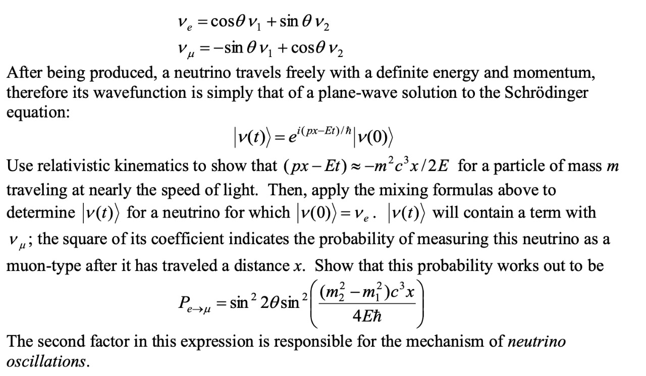
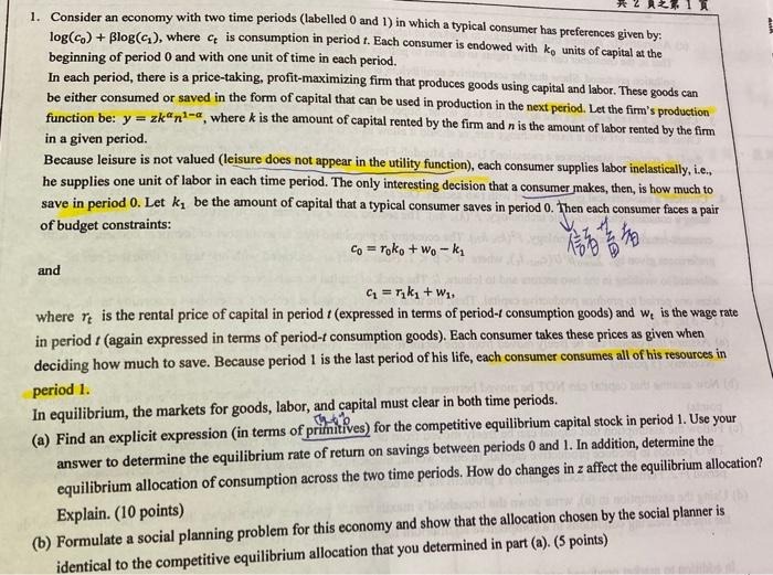
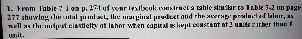
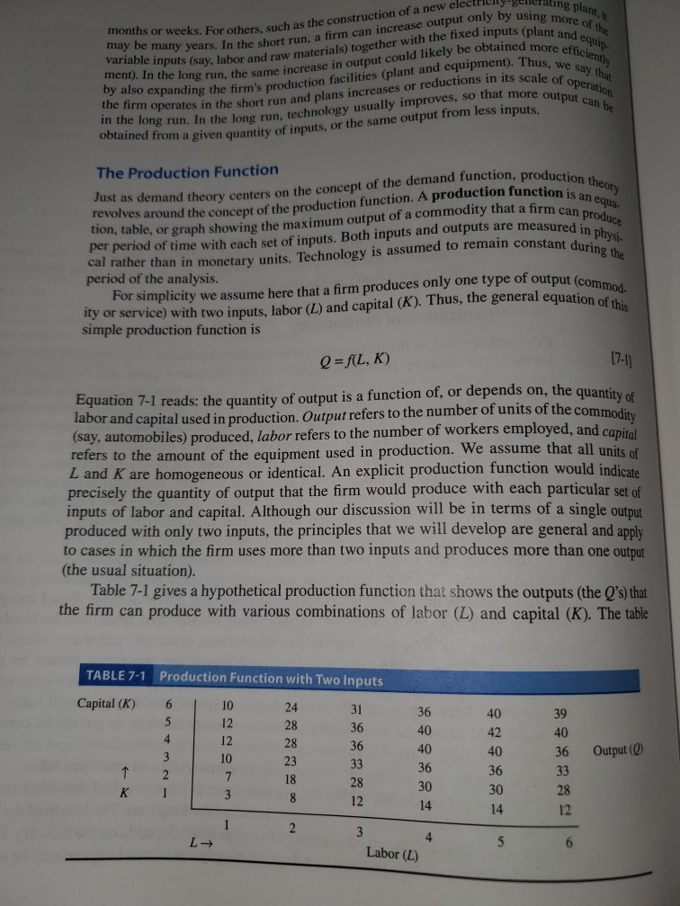
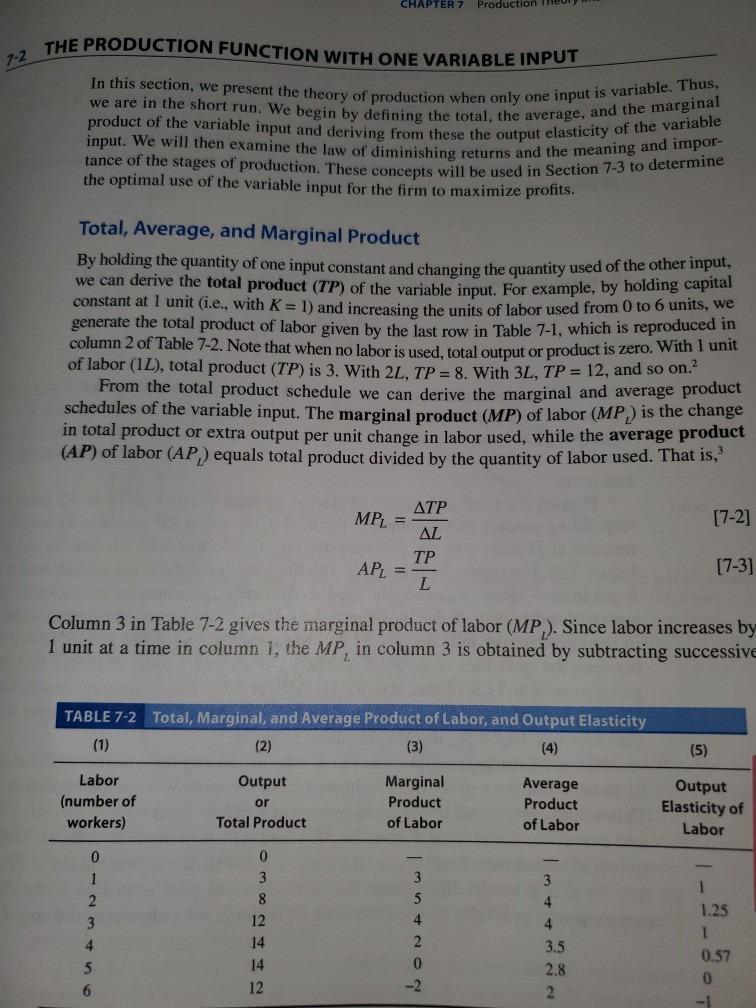
Ve = cosOv, + sin 0 v2 Vu =-sin 0 v1 + cos0 v2 After being produced, a neutrino travels freely with a definite energy and momentum, therefore its wavefunction is simply that of a plane-wave solution to the Schrodinger equation: [v(t)) = ei( px-Et)in| v(0)) Use relativistic kinematics to show that (px - Et) ~ -m c'x/2E for a particle of mass m traveling at nearly the speed of light. Then, apply the mixing formulas above to determine v(t) for a neutrino for which v(0)) = Ve . v(t)) will contain a term with vu; the square of its coefficient indicates the probability of measuring this neutrino as a muon-type after it has traveled a distance x. Show that this probability works out to be Peru = sin 2 20sin 2 (mz -m? )c'x 4Eh The second factor in this expression is responsible for the mechanism of neutrino oscillations.1. Consider an economy with two time periods (labelled 0 and 1) in which a typical consumer has preferences given by: log(co) + Blog(c,), where c is consumption in period f. Each consumer is endowed with ko units of capital at the beginning of period 0 and with one unit of time in each period. In each period, there is a price-taking, profit-maximizing firm that produces goods using capital and labor. These goods can be either consumed or saved in the form of capital that can be used in production in the next period. Let the firm's production function be: y = zk'n'-", where k is the amount of capital rented by the firm and n is the amount of labor rented by the firm in a given period. Because leisure is not valued (leisure does not appear in the utility function), each consumer supplies labor inelastically, i.c. he supplies one unit of labor in each time period. The only interesting decision that a consumer makes, then, is how much to save in period 0. Let k, be the amount of capital that a typical consumer saves in period 0. Then each consumer faces a pair of budget constraints: Co = Toko + Wo - k1 and where r, is the rental price of capital in period / (expressed in terms of period- consumption goods) and w, is the wage rate in period / (again expressed in terms of period- consumption goods). Each consumer takes these prices as given when deciding how much to save. Because period 1 is the last period of his life, each consumer consumes all of his resources in period 1. In equilibrium, the markets for goods, labor, and capital must clear in both time periods. (a) Find an explicit expression (in terms of primitives) for the competitive equilibrium capital stock in period 1. Use your answer to determine the equilibrium rate of return on savings between periods 0 and 1. In addition, determine the equilibrium allocation of consumption across the two time periods. How do changes in z affect the equilibrium allocation? Explain. (10 points) (b) Formulate a social planning problem for this economy and show that the allocation chosen by the social planner is identical to the competitive equilibrium allocation that you determined in part (a). (5 points)1. From Table 7-1 on p. 274 of your textbook construct a table similar to Table 7-2 on page 277 showing the total product, the marginal product and the average product of labor, as well as the output elasticity of labor when capital is kept constant at 3 units rather than 1 unit.ting plant, in months or weeks. For others, such as the construction of a new elect may be many years. In the short run, a firm can increase output of my using more of , it variable inputs (say, labor and raw materials) together with the fixed inputs (plant and er the "CI. In the long run. The same increase in output could likely be obtained more efficient also expanding the firm's production facilities (plant and equipment). Thus, we say my the firm operates in the short run and plans increases or reductions in its scale of operahill in the long run. In the long run, technology usually improves, so that more output can on obtained from a given quantity of inputs, or the same output from less inputs. The Production Function Just as demand theory centers on the concept of the demand function, production theory, revolves around the concept of the production function. A production function is an equy tion, table, or graph showing the maximum output of a commodity that a firm can product per period of time with each set of inputs. Both inputs and outputs are measured in cal rather than in monetary units. Technology is assumed to remain constant during the period of the analysis. For simplicity we assume here that a firm produces only one type of output (commod ity or service) with two inputs, labor (L) and capital (K). Thus, the general equation of this simple production function is Q = AL, K) [7-1] Equation 7-1 reads: the quantity of output is a function of, or depends on, the quantity of labor and capital used in production. Output refers to the number of units of the commodity (say, automobiles) produced, labor refers to the number of workers employed, and capital refers to the amount of the equipment used in production. We assume that all units of L and K are homogeneous or identical. An explicit production function would indicate precisely the quantity of output that the firm would produce with each particular set of inputs of labor and capital. Although our discussion will be in terms of a single output produced with only two inputs, the principles that we will develop are general and apply to cases in which the firm uses more than two inputs and produces more than one output (the usual situation). Table 7-1 gives a hypothetical production function that shows the outputs (the Q's) that the firm can produce with various combinations of labor (L) and capital (K). The table TABLE 7-1 Production Function with Two Inputs Capital (K) 10 24 31 36 40 39 12 28 36 40 42 40 12 28 36 40 40 36 Output (() 10 23 33 - N W 36 36 33 18 28 30 30 28 12 14 14 12 2 3 L- 5 6 Labor (L)7-2 THE PRODUCTION FUNCTION WITH ONE VARIABLE INPUT In this section, we present the theory of production when only one input is variable. Thus, we are in the short run. We begin by defining the total, the average, and the marginal product of the variable input and deriving from these the output elasticity of the variable input. We will then examine the law of diminishing returns and the meaning and impor- tance of the stages of production. These concepts will be used in Section 7-3 to determine the optimal use of the variable input for the firm to maximize profits. Total, Average, and Marginal Product By holding the quantity of one input constant and changing the quantity used of the other input, we can derive the total product (TP) of the variable input. For example, by holding capital constant at 1 unit (i.e., with K = 1) and increasing the units of labor used from 0 to 6 units, we generate the total product of labor given by the last row in Table 7-1, which is reproduced in column 2 of Table 7-2. Note that when no labor is used, total output or product is zero. With 1 unit of labor (12), total product (TP) is 3. With 2L, TP = 8. With 3L, TP = 12, and so on. From the total product schedule we can derive the marginal and average product schedules of the variable input. The marginal product (MP) of labor (MP ) is the change in total product or extra output per unit change in labor used, while the average product (AP) of labor (AP ) equals total product divided by the quantity of labor used. That is,' ATP MPL. = [7-2] AL TP APL = [7-3] L Column 3 in Table 7-2 gives the marginal product of labor (MP,). Since labor increases by 1 unit at a time in column 1, the MP, in column 3 is obtained by subtracting successive TABLE 7-2 Total, Marginal, and Average Product of Labor, and Output Elasticity (1) (2) (3) (4) (5) Labor Output Marginal Average Output (number of or Product Product Elasticity of workers) Total Product of Labor of Labor Labor 00 W E W N - O 1.25 12 NONAVIWI 1 14 3.5 0.57 aut 14 2.8 N