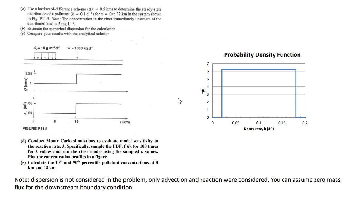
(a) Use a backward-difference scheme (Ax = 0.5 km) to determine the steady-state distribution of a pollutant (k = 0.1d-b) for x = 0 to 32 km in the system shown in Fig. P11.5. Note: The concentration in the river immediately upstream of the distributed load is 5 mg L- (b) Estimate the numerical dispersion for the calculation. (c) Compare your results with the analytical solution S-10 gm W = 1000 kg - Probability Density Function 7 2.25 6 5 (cms) 4 ) 3 60 2 1 20 0 16 (km) 0 0.05 0.15 0.2 FIGURE P11.5 0.1 Decay rate, k (d) (d) Conduct Monte Carlo simulations to evaluate model sensitivity to the reaction rate, k. Specifically, sample the PDF, f(k), for 100 times for k values and run the river model using the sampled k values. Plot the concentration profiles in a figure. (e) Calculate the 10th and 90th percentile pollutant concentrations at 8 km and 18 km. Note: dispersion is not considered in the problem, only advection and reaction were considered. You can assume zero mass flux for the downstream boundary condition