a working fortran code is required. it should a fortran code file with .F95

this is all the information

the first code is wrong. we have to correct it to make it a running code.

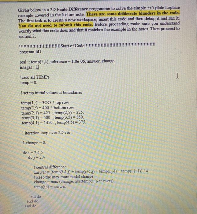
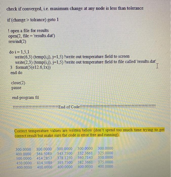
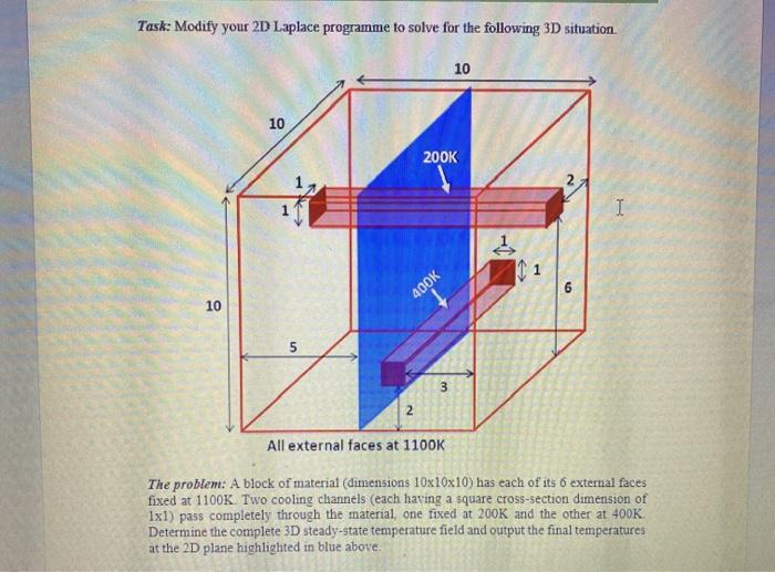
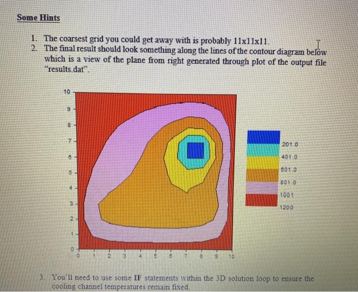
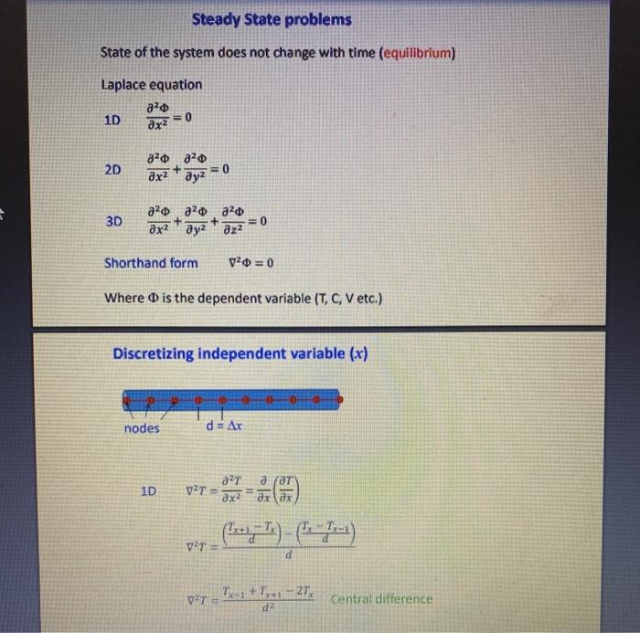
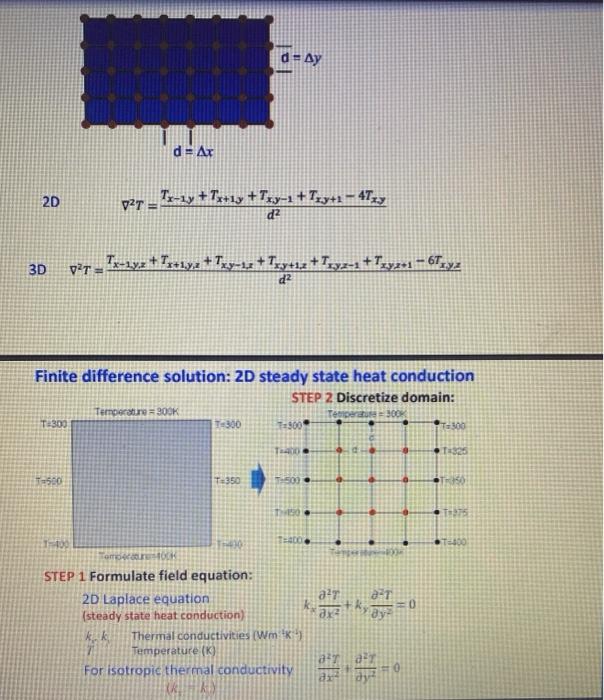
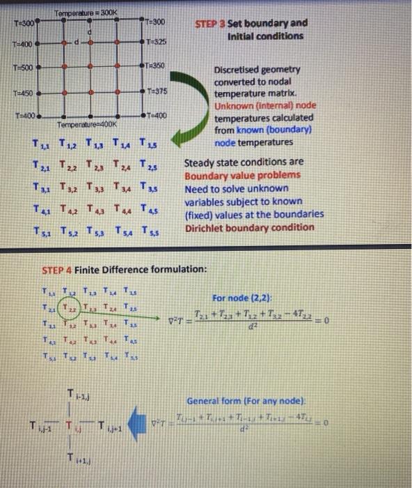
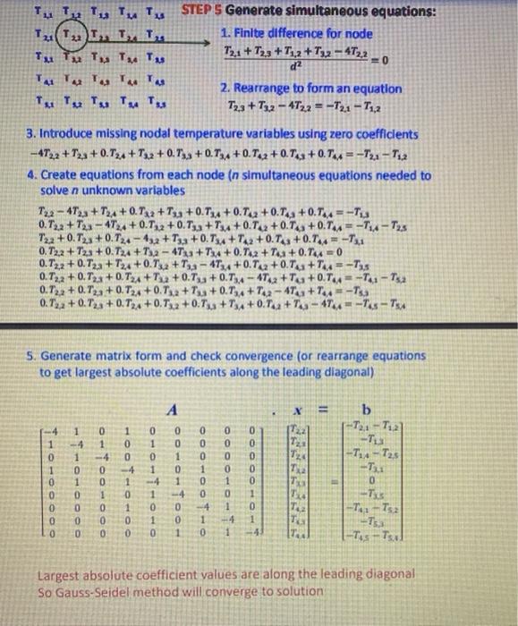
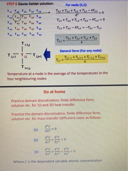
Given below is a 2D Finite Difference programme to solve the simple 55 plate Laplace example covered in the lecture note. There are some deliberate blunders in the code. The first task is to create a new workspace, insert this code and then debug it and run it You do not need to submit this code. Before proceeding make sure you understand exactly what this code does and that it matches the example in the notes. Then proceed to section 2. !!!!Start of Code!!!!!!! program fd1 real temp(5,4), tolerance = 1.0e-06, answer. change integer : ij I Izero all TEMPS temp = 0. I set up initial values at boundaries temp(1,5) = 300. ! top row temp(5.) = 400. I bottom row temp(2,1)= 425.; temp(2,5) = 325. temp(3.1) = 500.; temp(3,5) = 350. temp(4.1) = 1450. ; temp(4,5) = 375. ! iteration loop over 2D i&i 1 change = 0. do i = 2,4,5 doj= 2,4 I central difference answer =(temp(i-1.j) + temp(i+1.j) + temp(ij-1) + temp(1.j-1))/4. ! keep the maximum nodal change change = max (change, abs(temp(1.j)-answer)) temp(ij) = answer end do end do end do check if converged, i.e. maximum change at any node is less than tolerance if (change > tolrance) goto 1 I open a file for results open(2, file = 'results.dat') rewind(2) doi= 1,5,1 write(6,3) (temp(ij).j=1,5) !write out temperature field to screen write(2,3) (temp(ij), j=1,5) !write out temperature field to file called 'results.dat 3 format(5(e12.6,1x)) I end do close(2) pause end program fd !!!!!!!!!End of Code!!!!!!!!! Correct temperature values are written below (don't spend too much time trying to get correct result but make sure the code is error free and running) 300.0000 300.0000 300.0000 300.0000 400.0000 364.5089 343.7500 332.3661 500.0000 414.2857 378.1250 360.7143 450.0000 414.5089393.7500 382.3661 400.0000 400.0000 400.0000 400.0000 300.0000 325.0000 350.0000 375.0000 400.0000 Task: Modify your 2D Laplace programme to solve for the following 3D situation 10 10 200K I 11 400K 10 3 All external faces at 1100K The problem: A block of material (dimensions 10x10x10) has each of its 6 external faces fixed at 1100K. Two cooling channels (each having a square cross-section dimension of 1xl) pass completely through the material, one fixed at 200K and the other at 400K Determine the complete 3D steady-state temperature field and output the final temperatures at the 2D plane highlighted in blue above. Some Hints 1. The coarsest grid you could get away with is probably 11x11x11. 2. The final result should look something along the lines of the contour diagram below which is a view of the plane from right generated through plot of the output file "results.dat". 10 9 8 2010 8 4010 601.0 5 8010 1001 3 1200 N 9 10 3. You'll need to use some IF statements within the 3D solution loop to ensure the cooling channel temperatures remain fixed. Steady State problems State of the system does not change with time (equilibrium) Laplace equation ao =0 ax ? 1D 2D ? ? + 2 ? = 0 3D ao 220 ad + ax2 z? + =0 Shorthand form v2 = 0 Where is the dependent variable (T, C, V etc.) Discretizing independent variable (x) nodes d= Ar 1D VT 32T 3x? a 7a7 xlax VT Capa) d VT = T-1+7+127, d Central difference d = ay d= Ar 2D v2T = Tu-1y Tx+13 +Try-1 +Try+1 - 4723 d2 3D pit - Tu-14.2 +Tx=19.2 + Twy-u2+Try+12 +1.72-1 +14731 - 6Try2 d? Finite difference solution: 2D steady state heat conduction STEP 2 Discretize domain: Temperature 300K 300 T:300 300 T3000 7.300 T40 11325 7500 T-350 500 TH10 00 2.1 100 Tomberok STEP 1 Formulate field equation: 2D Laplace equation (steady state heat conduction) kk Thermal conductivities (Wm') Temperature (K) For isotropic thermal conductivity CRM ay ar ay Temperature = 300K T=300 T-300 STEP 3 Set boundary and Initial conditions T-400 T2825 T500 OT-350 T-450 T-375 T=400& T-400 Temperature 400K T 11 T 1,2 T13 Tu Tu T2,1 T2,2 T2 T34 T25 T3,1 T2, T3, T4 T3,5 T4 T4 T43 T4 T4,5 Discretised geometry converted to nodal temperature matrix Unknown (internal) node temperatures calculated from known (boundary) node temperatures Steady state conditions are Boundary value problems Need to solve unknown variables subject to known (fixed) values at the boundaries Dirichlet boundary condition T5 T5,2 15, T54 TSS STEP 4 Finite Difference formulation: 13 12 For node (2,2) Tz + Zza + Tuz + 12 - 4T22_ Tu Tu Tu Tu Tu Tz Tu Tu 1:2 . Tu Ta TT VAT 0 dz T- General form (For any node) TI-T40 d T, 0 Tv VET Tu 1, 1TT, STEPS Generate simultaneous equations: Ti (T2) I T. Tu 1. Finite difference for node Tu Tu Tu Te Tu 72,1 +T2,3 +7.,2+1;2 - 4T2,2 d2 =0 TATT 2. Rearrange to form an equation Tu Tu Tu Tu Tos T33 +73.2 - 4T2,2 = -12.1 -T,2 3. Introduce missing nodal temperature variables using zero coefficients -4T22 +12 + 0.724 + 742 +0.74 +0.74 +0. T-2 +0. T +0. Tu = -1,2 - T12 4. Create equations from each node (n simultaneous equations needed to solve n unknown variables T22 - 4T +T24 +0.7x2 +T33 +0.734 +0. Tu +0. Tag +0.74 = -Tua 0.722 +T22 - 1724 +0.T22 +0. Ta +44 +0.74 +0.7.3 +0.74 = -1.4-Tys T22 +0.7 +0.734 - 17,2 +T3a +0.734 + T. +0.73 +0.74 -7,1 0.T22 +T2,3 +0.T24 + 732 - 4T23 +74+0. T-2 + Ta +0. Tu = 0 0.T2,2 +0.Tza+T24 +0.75 +Tua - 4734 +0.74 +0. Tu + = -Ts 0.T22 +0.722 +0.T24 +T +0.7,3 +0.734 - 47.2 +T3 +0.7.4 = -2 - Tsa 0.722 +0.72a + 0.724 +0.732 +7 + 0.734 +T2 - 4T + T - 0.722 +0.729 +0.724 +0.Tsx2 +0.73 +34 +0. Tu Tu -474 -Tus - Tsu 5. Generate matrix form and check convergence (or rearrange equations to get largest absolute coefficients along the leading diagonal) X 1 4 1 1 4 1 1 OOOOOO OOOOOO 0 1 0 1 4 1 0 1 0 OOOOO CO-OTOO- OOOOO b [-T2-T -T -714- Tas -Tu 0 T22 7 T22 Tua TO -OOOOO OOOOOO OOOOOO 1 4 -Tus T TG -Tu-T2 -4 1 1 -4 LTS 1 -Tas - Tv Largest absolute coefficient values are along the leading diagonal So Gauss-Seidel method will converge to solution STEP 6 Gauss-Seidel solution: T211,2 Tas T Tas Tu Tu Tu Tu Tas Tas Tu Tas Tas Tu Tu Tu Te Tu For node (2,2): T21 + T2a + Tu2 +T2,2 - 4T22 = 0 d? 72,1+T23 +7,2+1,2-472,2 = 0 T22+T32 - 4T22 = -T21-T12 T2.1+T22 +T12 +T32 TH 72,2 4 General form (For any node): , + Ty = 4 T+1, Temperature at a node is the average of the temperatures in the four neighbouring nodes Do at home Practice domain discretization, finite difference form, solution etc. for 1D and 3D heat transfer Practice the domain discretization, finite difference form, solution etc. for mass transfer (diffusion) cases as follows: 1D ac ax? ac ac + =0 ax ay? 2D 3D 20 ac 2.c + ex ay az 0 Where Cis the dependent variable atomic concentration Given below is a 2D Finite Difference programme to solve the simple 55 plate Laplace example covered in the lecture note. There are some deliberate blunders in the code. The first task is to create a new workspace, insert this code and then debug it and run it You do not need to submit this code. Before proceeding make sure you understand exactly what this code does and that it matches the example in the notes. Then proceed to section 2. !!!!Start of Code!!!!!!! program fd1 real temp(5,4), tolerance = 1.0e-06, answer. change integer : ij I Izero all TEMPS temp = 0. I set up initial values at boundaries temp(1,5) = 300. ! top row temp(5.) = 400. I bottom row temp(2,1)= 425.; temp(2,5) = 325. temp(3.1) = 500.; temp(3,5) = 350. temp(4.1) = 1450. ; temp(4,5) = 375. ! iteration loop over 2D i&i 1 change = 0. do i = 2,4,5 doj= 2,4 I central difference answer =(temp(i-1.j) + temp(i+1.j) + temp(ij-1) + temp(1.j-1))/4. ! keep the maximum nodal change change = max (change, abs(temp(1.j)-answer)) temp(ij) = answer end do end do end do check if converged, i.e. maximum change at any node is less than tolerance if (change > tolrance) goto 1 I open a file for results open(2, file = 'results.dat') rewind(2) doi= 1,5,1 write(6,3) (temp(ij).j=1,5) !write out temperature field to screen write(2,3) (temp(ij), j=1,5) !write out temperature field to file called 'results.dat 3 format(5(e12.6,1x)) I end do close(2) pause end program fd !!!!!!!!!End of Code!!!!!!!!! Correct temperature values are written below (don't spend too much time trying to get correct result but make sure the code is error free and running) 300.0000 300.0000 300.0000 300.0000 400.0000 364.5089 343.7500 332.3661 500.0000 414.2857 378.1250 360.7143 450.0000 414.5089393.7500 382.3661 400.0000 400.0000 400.0000 400.0000 300.0000 325.0000 350.0000 375.0000 400.0000 Task: Modify your 2D Laplace programme to solve for the following 3D situation 10 10 200K I 11 400K 10 3 All external faces at 1100K The problem: A block of material (dimensions 10x10x10) has each of its 6 external faces fixed at 1100K. Two cooling channels (each having a square cross-section dimension of 1xl) pass completely through the material, one fixed at 200K and the other at 400K Determine the complete 3D steady-state temperature field and output the final temperatures at the 2D plane highlighted in blue above. Some Hints 1. The coarsest grid you could get away with is probably 11x11x11. 2. The final result should look something along the lines of the contour diagram below which is a view of the plane from right generated through plot of the output file "results.dat". 10 9 8 2010 8 4010 601.0 5 8010 1001 3 1200 N 9 10 3. You'll need to use some IF statements within the 3D solution loop to ensure the cooling channel temperatures remain fixed. Steady State problems State of the system does not change with time (equilibrium) Laplace equation ao =0 ax ? 1D 2D ? ? + 2 ? = 0 3D ao 220 ad + ax2 z? + =0 Shorthand form v2 = 0 Where is the dependent variable (T, C, V etc.) Discretizing independent variable (x) nodes d= Ar 1D VT 32T 3x? a 7a7 xlax VT Capa) d VT = T-1+7+127, d Central difference d = ay d= Ar 2D v2T = Tu-1y Tx+13 +Try-1 +Try+1 - 4723 d2 3D pit - Tu-14.2 +Tx=19.2 + Twy-u2+Try+12 +1.72-1 +14731 - 6Try2 d? Finite difference solution: 2D steady state heat conduction STEP 2 Discretize domain: Temperature 300K 300 T:300 300 T3000 7.300 T40 11325 7500 T-350 500 TH10 00 2.1 100 Tomberok STEP 1 Formulate field equation: 2D Laplace equation (steady state heat conduction) kk Thermal conductivities (Wm') Temperature (K) For isotropic thermal conductivity CRM ay ar ay Temperature = 300K T=300 T-300 STEP 3 Set boundary and Initial conditions T-400 T2825 T500 OT-350 T-450 T-375 T=400& T-400 Temperature 400K T 11 T 1,2 T13 Tu Tu T2,1 T2,2 T2 T34 T25 T3,1 T2, T3, T4 T3,5 T4 T4 T43 T4 T4,5 Discretised geometry converted to nodal temperature matrix Unknown (internal) node temperatures calculated from known (boundary) node temperatures Steady state conditions are Boundary value problems Need to solve unknown variables subject to known (fixed) values at the boundaries Dirichlet boundary condition T5 T5,2 15, T54 TSS STEP 4 Finite Difference formulation: 13 12 For node (2,2) Tz + Zza + Tuz + 12 - 4T22_ Tu Tu Tu Tu Tu Tz Tu Tu 1:2 . Tu Ta TT VAT 0 dz T- General form (For any node) TI-T40 d T, 0 Tv VET Tu 1, 1TT, STEPS Generate simultaneous equations: Ti (T2) I T. Tu 1. Finite difference for node Tu Tu Tu Te Tu 72,1 +T2,3 +7.,2+1;2 - 4T2,2 d2 =0 TATT 2. Rearrange to form an equation Tu Tu Tu Tu Tos T33 +73.2 - 4T2,2 = -12.1 -T,2 3. Introduce missing nodal temperature variables using zero coefficients -4T22 +12 + 0.724 + 742 +0.74 +0.74 +0. T-2 +0. T +0. Tu = -1,2 - T12 4. Create equations from each node (n simultaneous equations needed to solve n unknown variables T22 - 4T +T24 +0.7x2 +T33 +0.734 +0. Tu +0. Tag +0.74 = -Tua 0.722 +T22 - 1724 +0.T22 +0. Ta +44 +0.74 +0.7.3 +0.74 = -1.4-Tys T22 +0.7 +0.734 - 17,2 +T3a +0.734 + T. +0.73 +0.74 -7,1 0.T22 +T2,3 +0.T24 + 732 - 4T23 +74+0. T-2 + Ta +0. Tu = 0 0.T2,2 +0.Tza+T24 +0.75 +Tua - 4734 +0.74 +0. Tu + = -Ts 0.T22 +0.722 +0.T24 +T +0.7,3 +0.734 - 47.2 +T3 +0.7.4 = -2 - Tsa 0.722 +0.72a + 0.724 +0.732 +7 + 0.734 +T2 - 4T + T - 0.722 +0.729 +0.724 +0.Tsx2 +0.73 +34 +0. Tu Tu -474 -Tus - Tsu 5. Generate matrix form and check convergence (or rearrange equations to get largest absolute coefficients along the leading diagonal) X 1 4 1 1 4 1 1 OOOOOO OOOOOO 0 1 0 1 4 1 0 1 0 OOOOO CO-OTOO- OOOOO b [-T2-T -T -714- Tas -Tu 0 T22 7 T22 Tua TO -OOOOO OOOOOO OOOOOO 1 4 -Tus T TG -Tu-T2 -4 1 1 -4 LTS 1 -Tas - Tv Largest absolute coefficient values are along the leading diagonal So Gauss-Seidel method will converge to solution STEP 6 Gauss-Seidel solution: T211,2 Tas T Tas Tu Tu Tu Tu Tas Tas Tu Tas Tas Tu Tu Tu Te Tu For node (2,2): T21 + T2a + Tu2 +T2,2 - 4T22 = 0 d? 72,1+T23 +7,2+1,2-472,2 = 0 T22+T32 - 4T22 = -T21-T12 T2.1+T22 +T12 +T32 TH 72,2 4 General form (For any node): , + Ty = 4 T+1, Temperature at a node is the average of the temperatures in the four neighbouring nodes Do at home Practice domain discretization, finite difference form, solution etc. for 1D and 3D heat transfer Practice the domain discretization, finite difference form, solution etc. for mass transfer (diffusion) cases as follows: 1D ac ax? ac ac + =0 ax ay? 2D 3D 20 ac 2.c + ex ay az 0 Where Cis the dependent variable atomic concentration