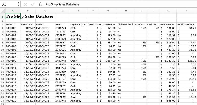
A1 x fx Pro Shop Sales Database B D E F G H K L 1 Pro Shop Sales Database 2 3 TransID 4 P000100 5 P000101 6 P000102 7 P000103 8 P000104 9 P000105 10 PO00106 11 P000107 12 P000108 13 PO00109 14 P000110 15 PO00111 16 P000112 17 PO00113 18 P000114 19 PO00115 20 P000116 21 P000117 22 PO00118 23 P000119 24 P000120 25 TransDate EMP-ID 10/3/22 EMP-00076 10/3/22 EMP-00038 10/3/22 EMP-00024 10/5/22 EMP-00015 10/6/22 EMP-00026 10/12/22 EMP-00076 10/16/22 EMP-00038 10/22/22 EMP-00024 10/25/22 EMP-00015 11/2/22 EMP-00026 11/7/22 EMP-00076 11/10/22 EMP-00038 11/13/22 EMP-00024 11/23/22 EMP-00015 12/13/22 EMP-00026 12/14/22 EMP-00076 12/16/22 EMP-00038 12/18/22 EMP-00024 12/24/22 EMP-00015 12/29/22 EMP-00026 12/31/22 EMP-00076 ItemID C884P23 T822248 F232P37 C583K29 F232P37 F375P67 X740029 T981011 C884P23 X487P48 R483P24 R483P24 X349R39 F833K19 R239157 C583K29 F375P67 X487P48 F833K19 F232P37 X487248 Payment Type Quantity GrossRevenue Club Member? Coupon Cash Disc Net Revenue TotalDiscounts Cash 3 $ 171.00 No 15% 5% $ 136.80 $ 34.20 Cash 2 $ 65.90 No $ 65.90 $ Apple Pay 1 $ 129.00 Yes $ 119.97 $ 9.03 Apple Pay 3 $ 177.00 No $ 177.00 $ Credit 3 $ 387.00 No 15% 5% $ 309.60 $ 77.40 Cash 3 $ 46.35 Yes 15% $ 36.15 $ 10.20 Apple Pay 1 S 453.00 Yes $ 421.29 $ 31.71 Credit 1 $ 12.00 No $ 12.00 $ Cash 2 $ 114.00 No 5% $ 108.30 $ 5.70 Credit 3 $ 1,257.00 No 10% $ 1,131.30 $ 125.70 Apple Pay 1 $ 2.00 No 10% $ 1.80 $ 0.20 Card 1 $ 2.00 Yes 15% $ 1.56 $ 0.44 Credit 3 $ 149.85 No 5% $ 142.36 $ 7.49 Apple Pay 3 $ 17.85 No 5% $ 16.96 $ 0.89 Card 2 $ 194.00 No 15% $ 164.90 $ 29.10 Card 1 $ 59.00 No $ 59.00 $ Cash 3 $ 46.35 No $ 46.35 $ Apple Pay 2 $ 838.00 Yes $ 779.34 $ 58.66 Apple Pay 4 $ 23.80 No $ 23.80 $ Card 1 $ 129.00 Yes $ 113.52 $ 15.48 Apple Pay 2 S 838.00 No $ 838.00 $ 5% A B 1 2 3 4 5 Field 6 7 Sum 8 Average 9 Count 10 Max 11 Min 2 Database functions allow for the user to specify criteria in one or more fields to explore the data with ease. When this is done, all the criteria must be evaluated to TRUE for the record to be included in the calculation. Using a table for the Excel Database allows you to add new records to the database easily and any database functions used on the table will automatically update. On the SalesData worksheet, convert the plain data set to an Excel table. Name the Excel table, Sales.Data, and then create a named range, Sales Database, for all of the data in the table, including the column headings. Copy the column headings from the SalesData table and paste them on the Database Totals worksheet, starting in cell A1 to setup the criteria area of for use in the Database functions. On the Database Totals worksheet, in cell B5, type NetRevenue for the field name that will be used in the database functions. In cells 37:B11, use the appropriate Database function to calculate the sum, average, count, max, and min of the NetRevenue field using the range A1:L2 as the criteria. Once all database functions have been created, use the criteria area to limit the calculations to those records with transaction dates after 11/15/2022 and with Apple Pay as the payment method. Finally, change the field being used in the calculations from NetRevenue to TatalDiscounts. 3 Excel's Recommended PivotTables feature allows you to easily explore data from many different perspectives with just a few clicks. Once created, they can be easily modified to improve readability and even changed to further explore the data. Using the data on the SalesData worksheet, use the Recommended PivotTable button on the Insert tab to create the Average of Cash Disc by Quantity PivotTable. ***************** If using a Mac, the Recommended PivotTable automatically created will need to be modified before moving forward. In the Pivot Table Fields pane, click to deselect TransDate. NetRevenue and EMP-ID. In the PivotTable Fields pane, drag Quantity to Rows, Club Member? to columns, and Cash Disc to Values Right-click the CashDisc field in the Values area, select Field Settings, and change the Summarize by function to Average. Configure the Pivot Table Options so that error values are shown as 0 In cell A4, replace Row Labels with Quantity Sold an in cell B3, replace Column Labels with Cash Discount? Remove the CashDisc field from the Values area and replace it with the TotalDiscounts field. Rename the worksheet to be TotalDiscountsBxQty. 4 A PivotTable is an interactive table that extracts, organizes, and summarizes source data. PivotTables are used for data analysis and looking for trends and patterns for decision-making purposes. The first step in creating a PivotTable is to select the data to be used and the location where it is to be created. Use the data in the Sales Data Excel Table to create a PivotTable on a new worksheet. Name the new worksheet PixatAnalysis, 5 Seeing how the Net Revenue breaks down into various groups can be easily done with PivotTables. Create a Pivot Table that displays the NetRevenue values with the TransDate field grouped into Years, Quarters, and Months as the Rows and the Payment Type as the columns. Use the ClubMember? field as the report filter and only show the data for club members. PivotTables can be made more user-friendly and provide additional insights into your data though various PivotTable configuration options. Create a Total Net Revenue Custom Name for the Sum of NetRevenue field and format the field as Accounting with 2 decimal places. In cell A4, replace Row Labels with Quarters by Year and in cell B3, replace Column Labels with Payment Type. Change the PivotTable so that it shows the Total Net Revenue as % of Grand Total. Apply the White, Pivot Style Light 23 to the PivotTable. 7 8 Slicers added to a PivotTable make it easy to apply various filters to the data. Insert an EMP-ID slicer to the PivotTable. Position the slicer so that the top-left corner is in cell G3 and then drag the bottom edge to adjust the height so that the extra white space is no longer visible. Do not drag it so far that you see a scroll bar on the right side. Modify the Header Caption of the slicer to be Employee and apply the White, Slicer Style Other 2. Use the slicer so that only the records for EMP-00024 are showing. As new transactions are recorded in the SalesData table, the Pivot Table can be easily refreshed to incorporate the new records into the analysis. Add the following data to row 25 of the Sales Data table: TransID P000121 TransDate 01/01/2023 EMP-ID EMP-00024 | ItemID T822748 PaymentType Cash Quantity 3 GrossRevenue 98.85 Club Member? Yes Coupon Cash Disc NetRevenue 98.85 TotalDiscounts 0 Refresh the Pivot Table so that the new transaction is included in the Analysis and then clear all PivotTable filters. Create a drill-down of the December, 2022 Apple Pay transactions onto a new worksheet and name the worksheet Apple Pay Transactions. 9 PivotCharts can add a visual component to your analysis with options to filter specific records. Create a PivotChart based on the data in the SalesData table. Start the analysis on a new worksheet, renamed to be RexenueByPaymentType The PivotChart should be a Pie Chart that shows the proportion of Net Revenue from each Payment Type. Use Years as the filter so that you can see the data for any given year. Move the Pie Chart to its own worksheet named, Revenue BxTyRePixatChart Edit the chart title to be Proportion of Revenue by Payment Type Use the Years Filter to only show transactions from 2022. A1 x fx Pro Shop Sales Database B D E F G H K L 1 Pro Shop Sales Database 2 3 TransID 4 P000100 5 P000101 6 P000102 7 P000103 8 P000104 9 P000105 10 PO00106 11 P000107 12 P000108 13 PO00109 14 P000110 15 PO00111 16 P000112 17 PO00113 18 P000114 19 PO00115 20 P000116 21 P000117 22 PO00118 23 P000119 24 P000120 25 TransDate EMP-ID 10/3/22 EMP-00076 10/3/22 EMP-00038 10/3/22 EMP-00024 10/5/22 EMP-00015 10/6/22 EMP-00026 10/12/22 EMP-00076 10/16/22 EMP-00038 10/22/22 EMP-00024 10/25/22 EMP-00015 11/2/22 EMP-00026 11/7/22 EMP-00076 11/10/22 EMP-00038 11/13/22 EMP-00024 11/23/22 EMP-00015 12/13/22 EMP-00026 12/14/22 EMP-00076 12/16/22 EMP-00038 12/18/22 EMP-00024 12/24/22 EMP-00015 12/29/22 EMP-00026 12/31/22 EMP-00076 ItemID C884P23 T822248 F232P37 C583K29 F232P37 F375P67 X740029 T981011 C884P23 X487P48 R483P24 R483P24 X349R39 F833K19 R239157 C583K29 F375P67 X487P48 F833K19 F232P37 X487248 Payment Type Quantity GrossRevenue Club Member? Coupon Cash Disc Net Revenue TotalDiscounts Cash 3 $ 171.00 No 15% 5% $ 136.80 $ 34.20 Cash 2 $ 65.90 No $ 65.90 $ Apple Pay 1 $ 129.00 Yes $ 119.97 $ 9.03 Apple Pay 3 $ 177.00 No $ 177.00 $ Credit 3 $ 387.00 No 15% 5% $ 309.60 $ 77.40 Cash 3 $ 46.35 Yes 15% $ 36.15 $ 10.20 Apple Pay 1 S 453.00 Yes $ 421.29 $ 31.71 Credit 1 $ 12.00 No $ 12.00 $ Cash 2 $ 114.00 No 5% $ 108.30 $ 5.70 Credit 3 $ 1,257.00 No 10% $ 1,131.30 $ 125.70 Apple Pay 1 $ 2.00 No 10% $ 1.80 $ 0.20 Card 1 $ 2.00 Yes 15% $ 1.56 $ 0.44 Credit 3 $ 149.85 No 5% $ 142.36 $ 7.49 Apple Pay 3 $ 17.85 No 5% $ 16.96 $ 0.89 Card 2 $ 194.00 No 15% $ 164.90 $ 29.10 Card 1 $ 59.00 No $ 59.00 $ Cash 3 $ 46.35 No $ 46.35 $ Apple Pay 2 $ 838.00 Yes $ 779.34 $ 58.66 Apple Pay 4 $ 23.80 No $ 23.80 $ Card 1 $ 129.00 Yes $ 113.52 $ 15.48 Apple Pay 2 S 838.00 No $ 838.00 $ 5% A B 1 2 3 4 5 Field 6 7 Sum 8 Average 9 Count 10 Max 11 Min 2 Database functions allow for the user to specify criteria in one or more fields to explore the data with ease. When this is done, all the criteria must be evaluated to TRUE for the record to be included in the calculation. Using a table for the Excel Database allows you to add new records to the database easily and any database functions used on the table will automatically update. On the SalesData worksheet, convert the plain data set to an Excel table. Name the Excel table, Sales.Data, and then create a named range, Sales Database, for all of the data in the table, including the column headings. Copy the column headings from the SalesData table and paste them on the Database Totals worksheet, starting in cell A1 to setup the criteria area of for use in the Database functions. On the Database Totals worksheet, in cell B5, type NetRevenue for the field name that will be used in the database functions. In cells 37:B11, use the appropriate Database function to calculate the sum, average, count, max, and min of the NetRevenue field using the range A1:L2 as the criteria. Once all database functions have been created, use the criteria area to limit the calculations to those records with transaction dates after 11/15/2022 and with Apple Pay as the payment method. Finally, change the field being used in the calculations from NetRevenue to TatalDiscounts. 3 Excel's Recommended PivotTables feature allows you to easily explore data from many different perspectives with just a few clicks. Once created, they can be easily modified to improve readability and even changed to further explore the data. Using the data on the SalesData worksheet, use the Recommended PivotTable button on the Insert tab to create the Average of Cash Disc by Quantity PivotTable. ***************** If using a Mac, the Recommended PivotTable automatically created will need to be modified before moving forward. In the Pivot Table Fields pane, click to deselect TransDate. NetRevenue and EMP-ID. In the PivotTable Fields pane, drag Quantity to Rows, Club Member? to columns, and Cash Disc to Values Right-click the CashDisc field in the Values area, select Field Settings, and change the Summarize by function to Average. Configure the Pivot Table Options so that error values are shown as 0 In cell A4, replace Row Labels with Quantity Sold an in cell B3, replace Column Labels with Cash Discount? Remove the CashDisc field from the Values area and replace it with the TotalDiscounts field. Rename the worksheet to be TotalDiscountsBxQty. 4 A PivotTable is an interactive table that extracts, organizes, and summarizes source data. PivotTables are used for data analysis and looking for trends and patterns for decision-making purposes. The first step in creating a PivotTable is to select the data to be used and the location where it is to be created. Use the data in the Sales Data Excel Table to create a PivotTable on a new worksheet. Name the new worksheet PixatAnalysis, 5 Seeing how the Net Revenue breaks down into various groups can be easily done with PivotTables. Create a Pivot Table that displays the NetRevenue values with the TransDate field grouped into Years, Quarters, and Months as the Rows and the Payment Type as the columns. Use the ClubMember? field as the report filter and only show the data for club members. PivotTables can be made more user-friendly and provide additional insights into your data though various PivotTable configuration options. Create a Total Net Revenue Custom Name for the Sum of NetRevenue field and format the field as Accounting with 2 decimal places. In cell A4, replace Row Labels with Quarters by Year and in cell B3, replace Column Labels with Payment Type. Change the PivotTable so that it shows the Total Net Revenue as % of Grand Total. Apply the White, Pivot Style Light 23 to the PivotTable. 7 8 Slicers added to a PivotTable make it easy to apply various filters to the data. Insert an EMP-ID slicer to the PivotTable. Position the slicer so that the top-left corner is in cell G3 and then drag the bottom edge to adjust the height so that the extra white space is no longer visible. Do not drag it so far that you see a scroll bar on the right side. Modify the Header Caption of the slicer to be Employee and apply the White, Slicer Style Other 2. Use the slicer so that only the records for EMP-00024 are showing. As new transactions are recorded in the SalesData table, the Pivot Table can be easily refreshed to incorporate the new records into the analysis. Add the following data to row 25 of the Sales Data table: TransID P000121 TransDate 01/01/2023 EMP-ID EMP-00024 | ItemID T822748 PaymentType Cash Quantity 3 GrossRevenue 98.85 Club Member? Yes Coupon Cash Disc NetRevenue 98.85 TotalDiscounts 0 Refresh the Pivot Table so that the new transaction is included in the Analysis and then clear all PivotTable filters. Create a drill-down of the December, 2022 Apple Pay transactions onto a new worksheet and name the worksheet Apple Pay Transactions. 9 PivotCharts can add a visual component to your analysis with options to filter specific records. Create a PivotChart based on the data in the SalesData table. Start the analysis on a new worksheet, renamed to be RexenueByPaymentType The PivotChart should be a Pie Chart that shows the proportion of Net Revenue from each Payment Type. Use Years as the filter so that you can see the data for any given year. Move the Pie Chart to its own worksheet named, Revenue BxTyRePixatChart Edit the chart title to be Proportion of Revenue by Payment Type Use the Years Filter to only show transactions from 2022