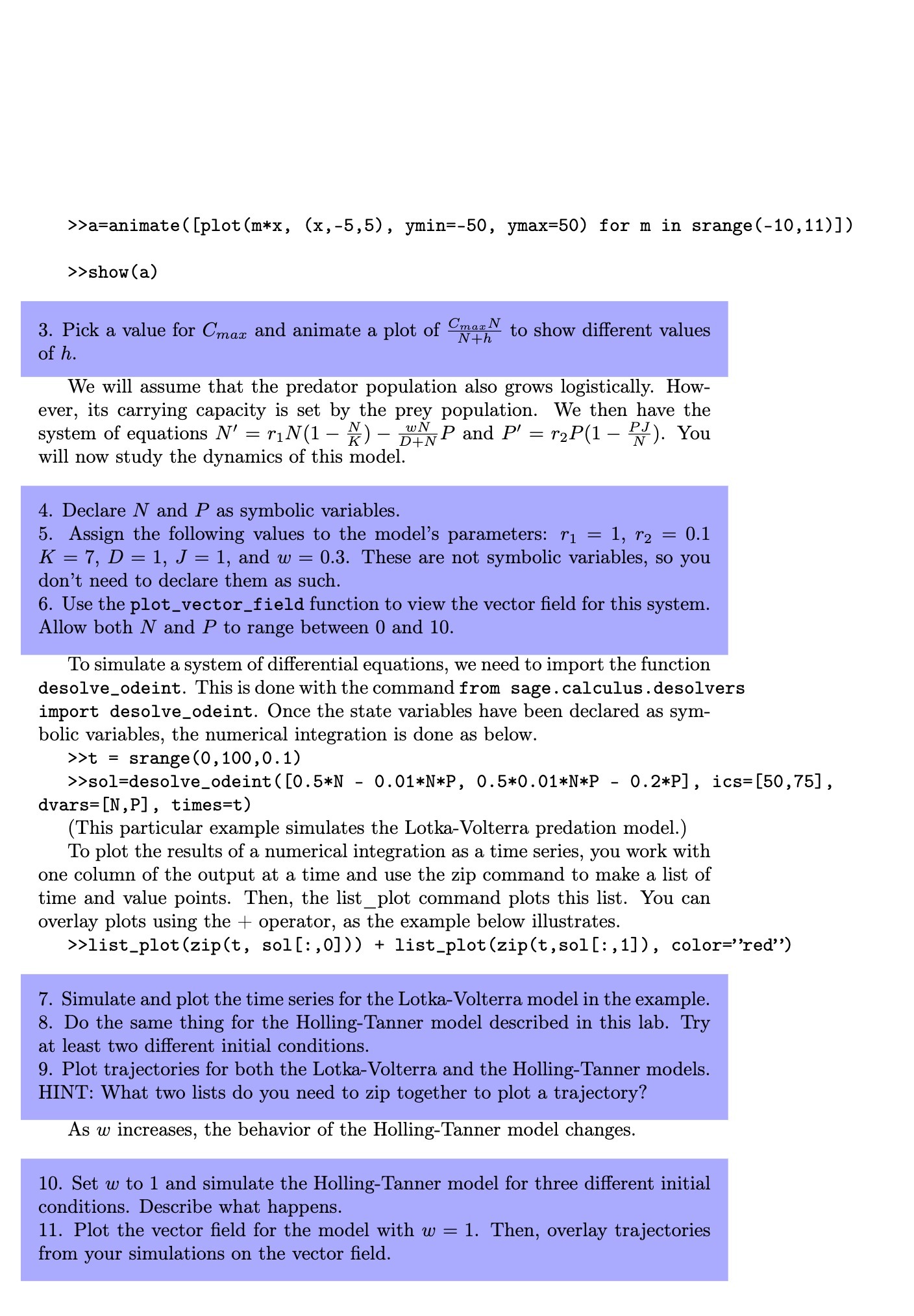
> >a=animate ( [plot (m*x, (x, -5,5), ymin=-50, ymax=50) for m in srange (-10, 11) ]) > >show (a) 3. Pick a value for Cmax and animate a plot of ward to show different values of h. We will assume that the predator population also grows logistically. How- ever, its carrying capacity is set by the prey population. We then have the system of equations N' = rIN(1 - A) - UN D+N P and P' = 12P(1 - N). You will now study the dynamics of this model. 4. Declare N and P as symbolic variables. 5. Assign the following values to the model's parameters: r1 = 1, r2 = 0.1 K = 7, D = 1, J = 1, and w = 0.3. These are not symbolic variables, so you don't need to declare them as such. 6. Use the plot_vector_field function to view the vector field for this system. Allow both N and P to range between 0 and 10. To simulate a system of differential equations, we need to import the function desolve_odeint. This is done with the command from sage . calculus . desolvers import desolve_odeint. Once the state variables have been declared as sym- bolic variables, the numerical integration is done as below. > >t = srange (0, 100, 0.1) >>sol=desolve_odeint ( [0.5*N - 0.01*N*P, 0.5*0. 01*N*P - 0.2*P], ics=[50, 75] , dvars= [N, P] , times=t) (This particular example simulates the Lotka-Volterra predation model.) To plot the results of a numerical integration as a time series, you work with one column of the output at a time and use the zip command to make a list of time and value points. Then, the list_plot command plots this list. You can overlay plots using the + operator, as the example below illustrates. > >list_plot (zip(t, sol[: , 0])) + list_plot(zip(t, sol[: , 1]), color="red") 7. Simulate and plot the time series for the Lotka-Volterra model in the example. 8. Do the same thing for the Holling-Tanner model described in this lab. Try at least two different initial conditions. 9. Plot trajectories for both the Lotka-Volterra and the Holling-Tanner models. HINT: What two lists do you need to zip together to plot a trajectory? As w increases, the behavior of the Holling-Tanner model changes. 10. Set w to 1 and simulate the Holling-Tanner model for three different initial conditions. Describe what happens. 11. Plot the vector field for the model with w = 1. Then, overlay trajectories from your simulations on the vector field