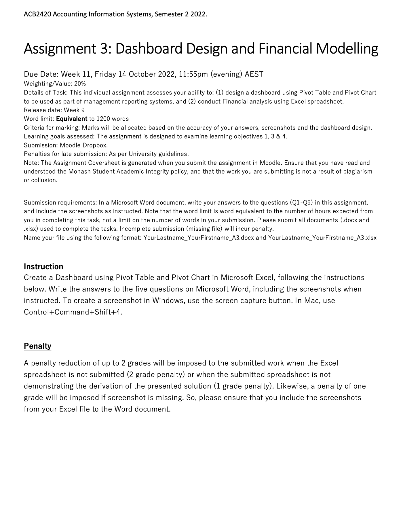
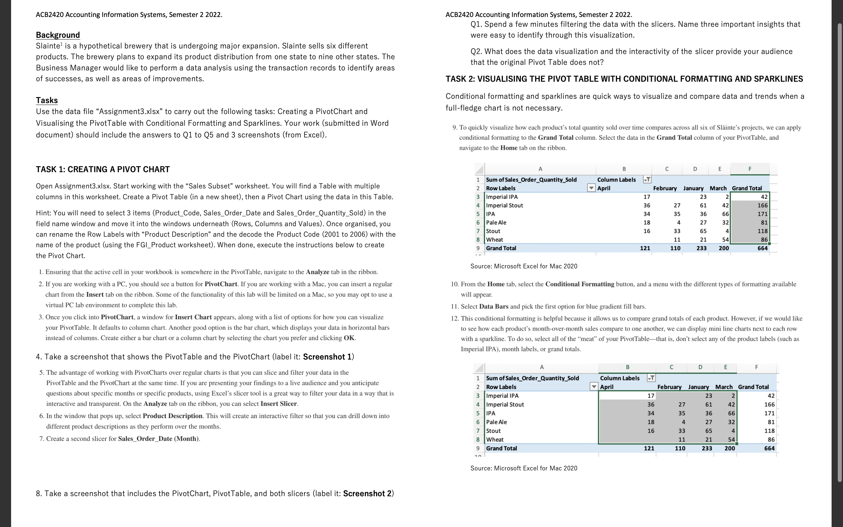
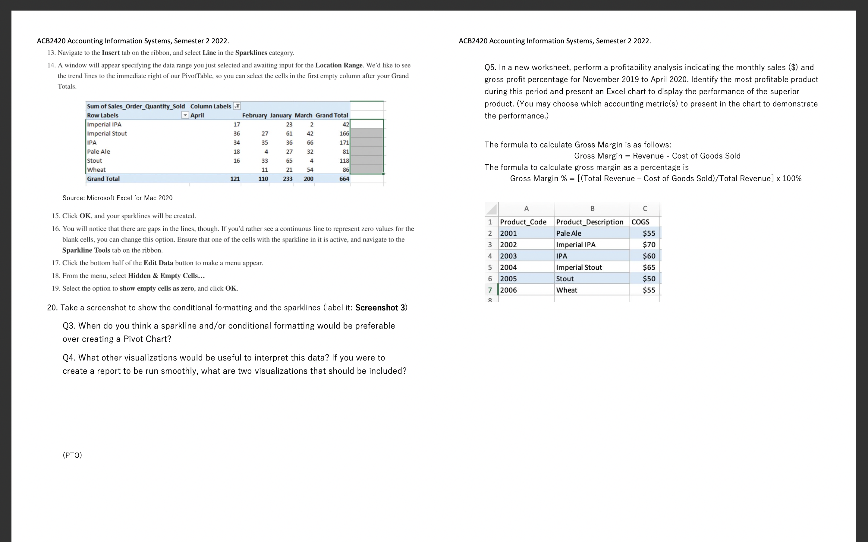
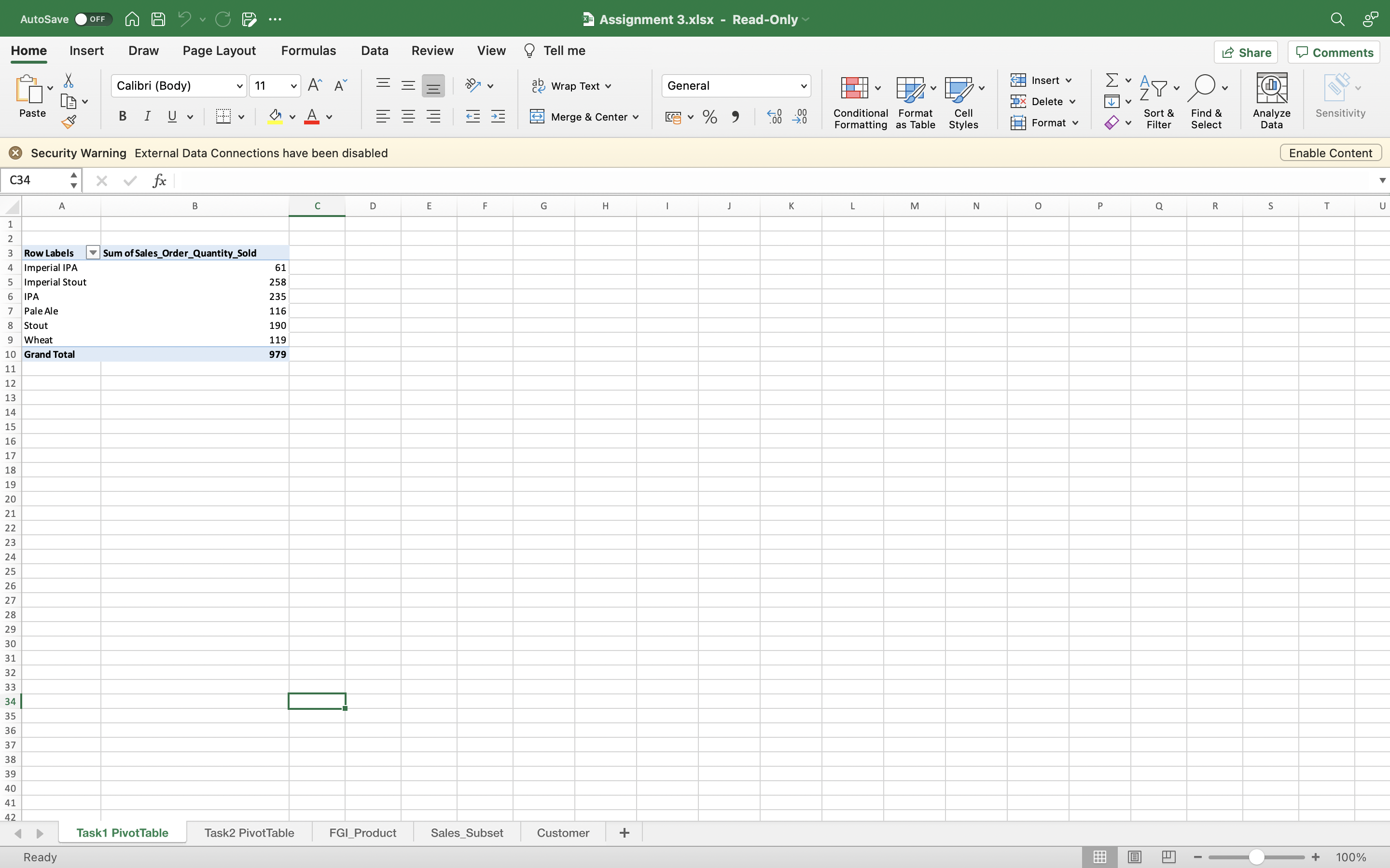
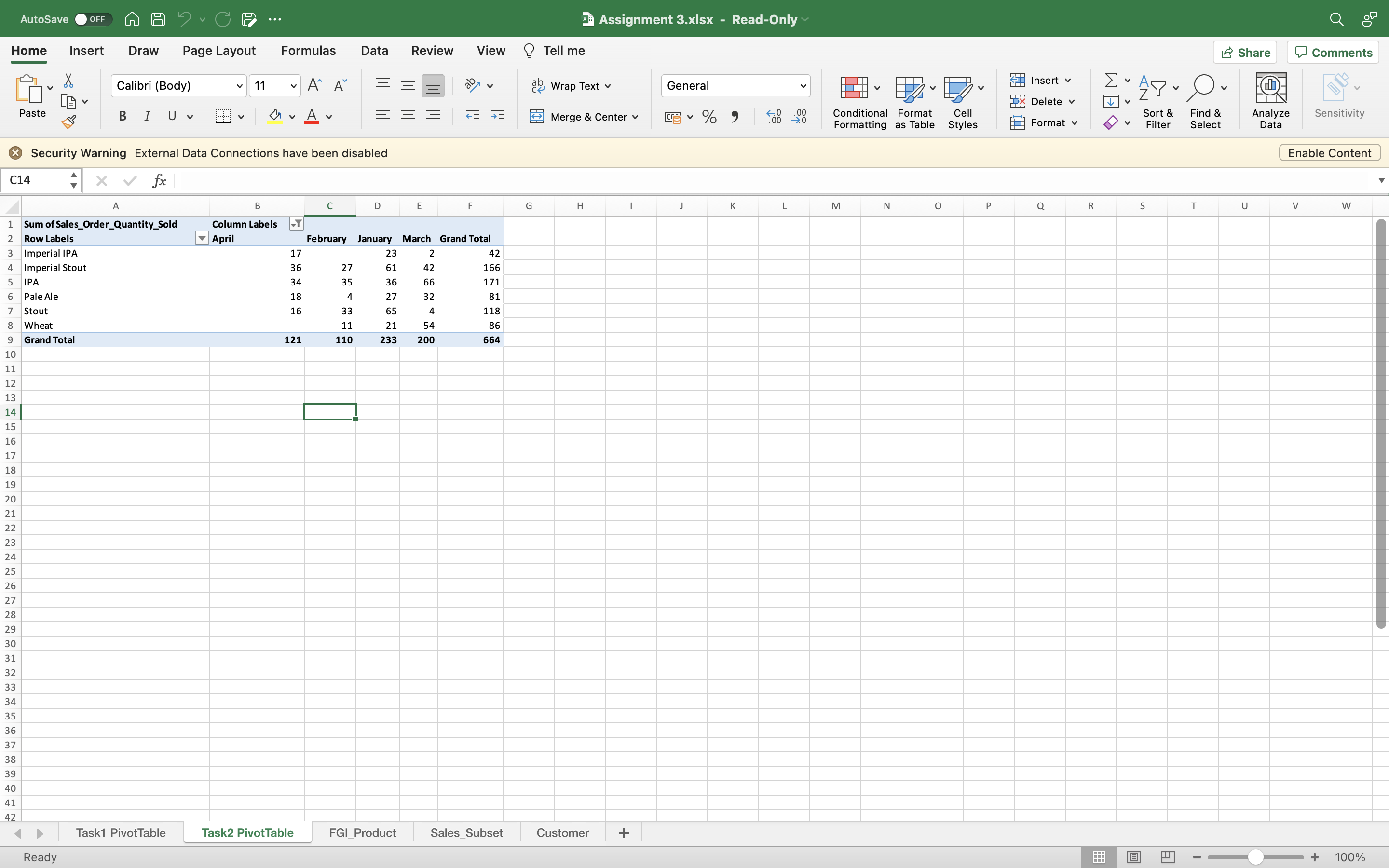
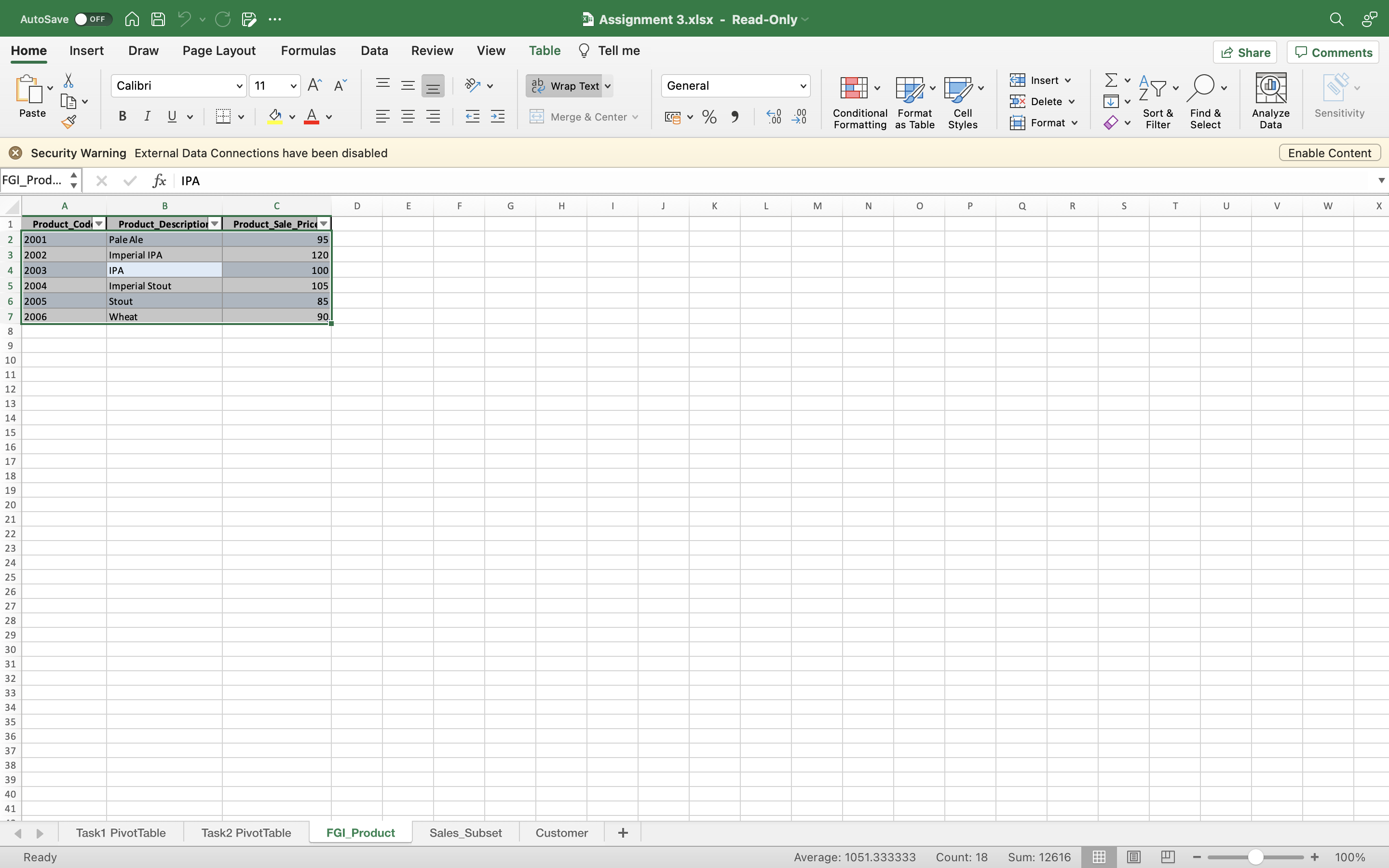
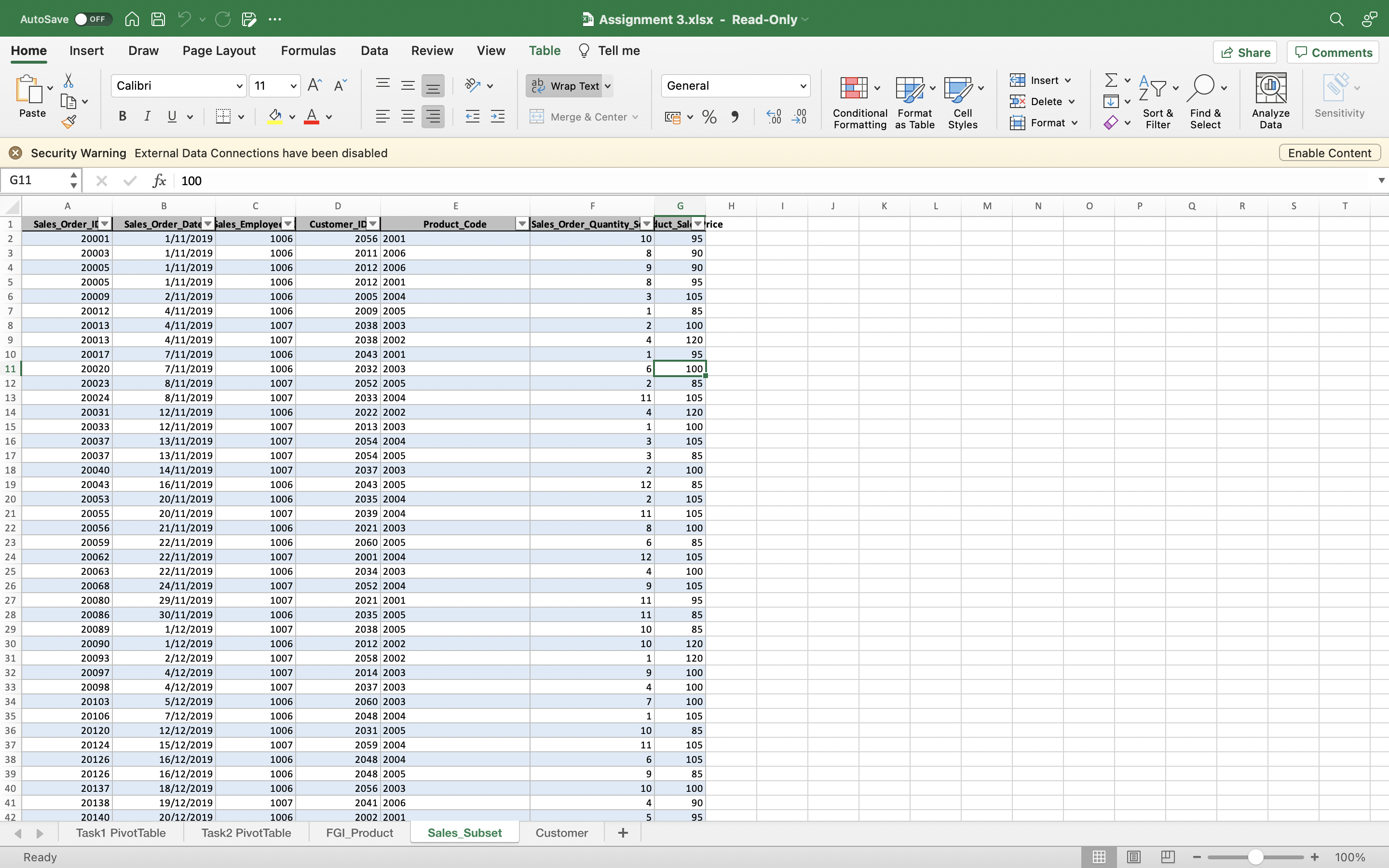
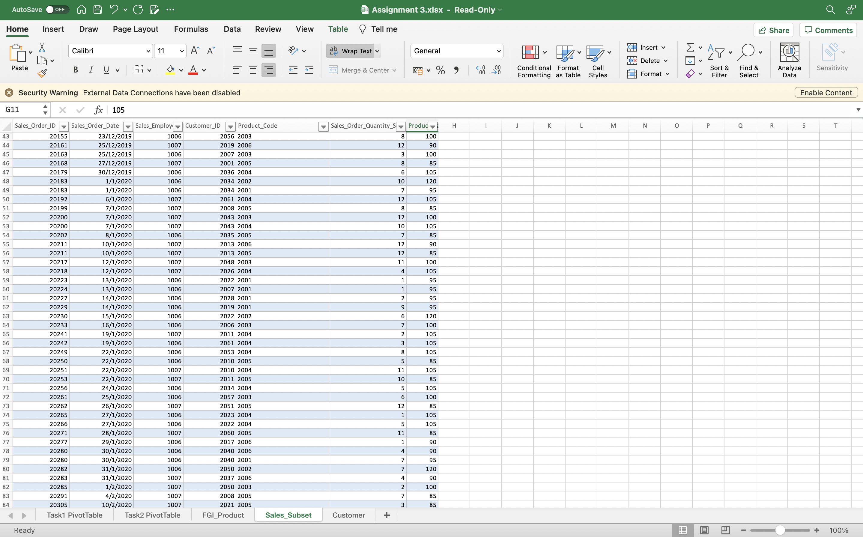
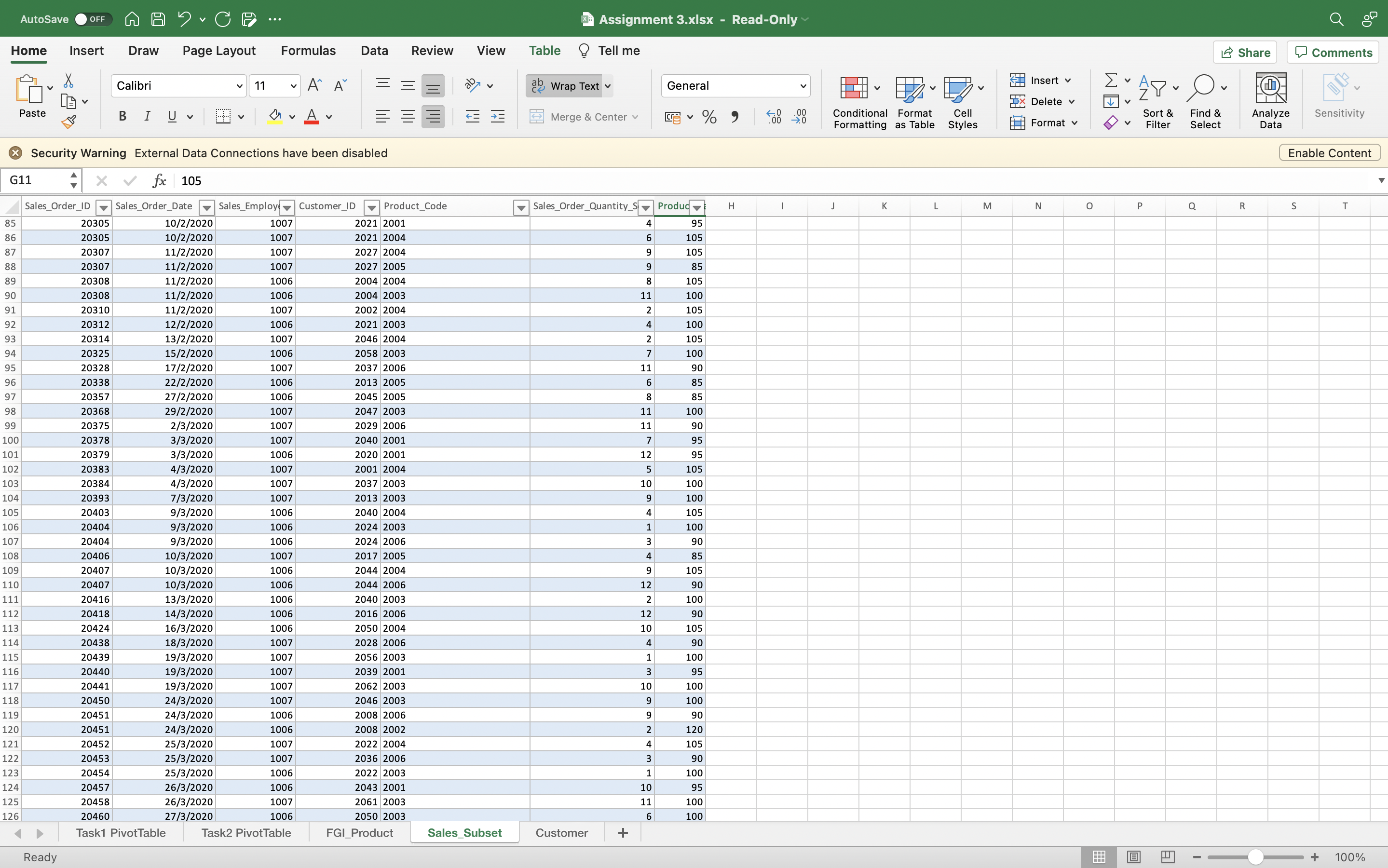
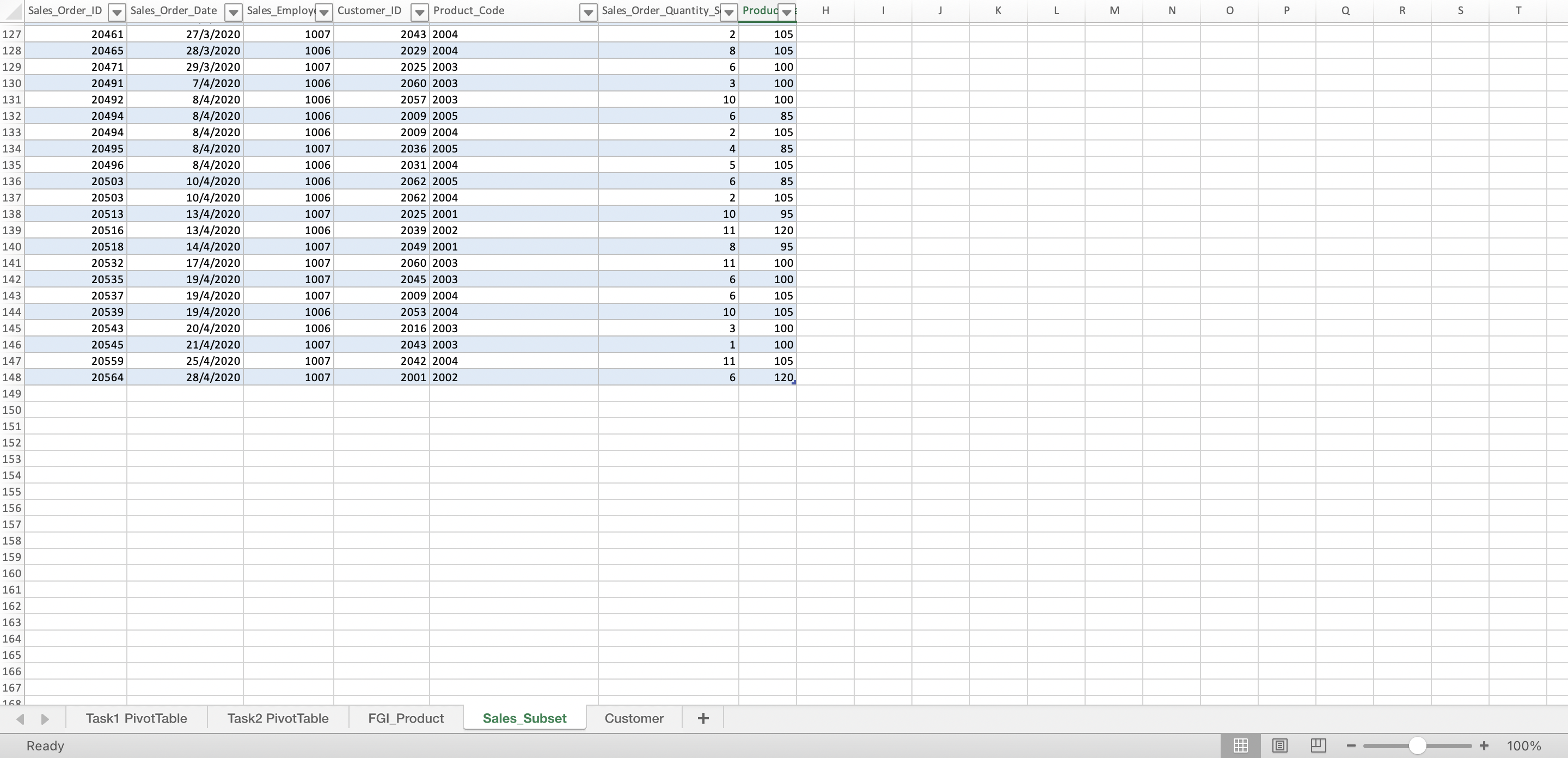
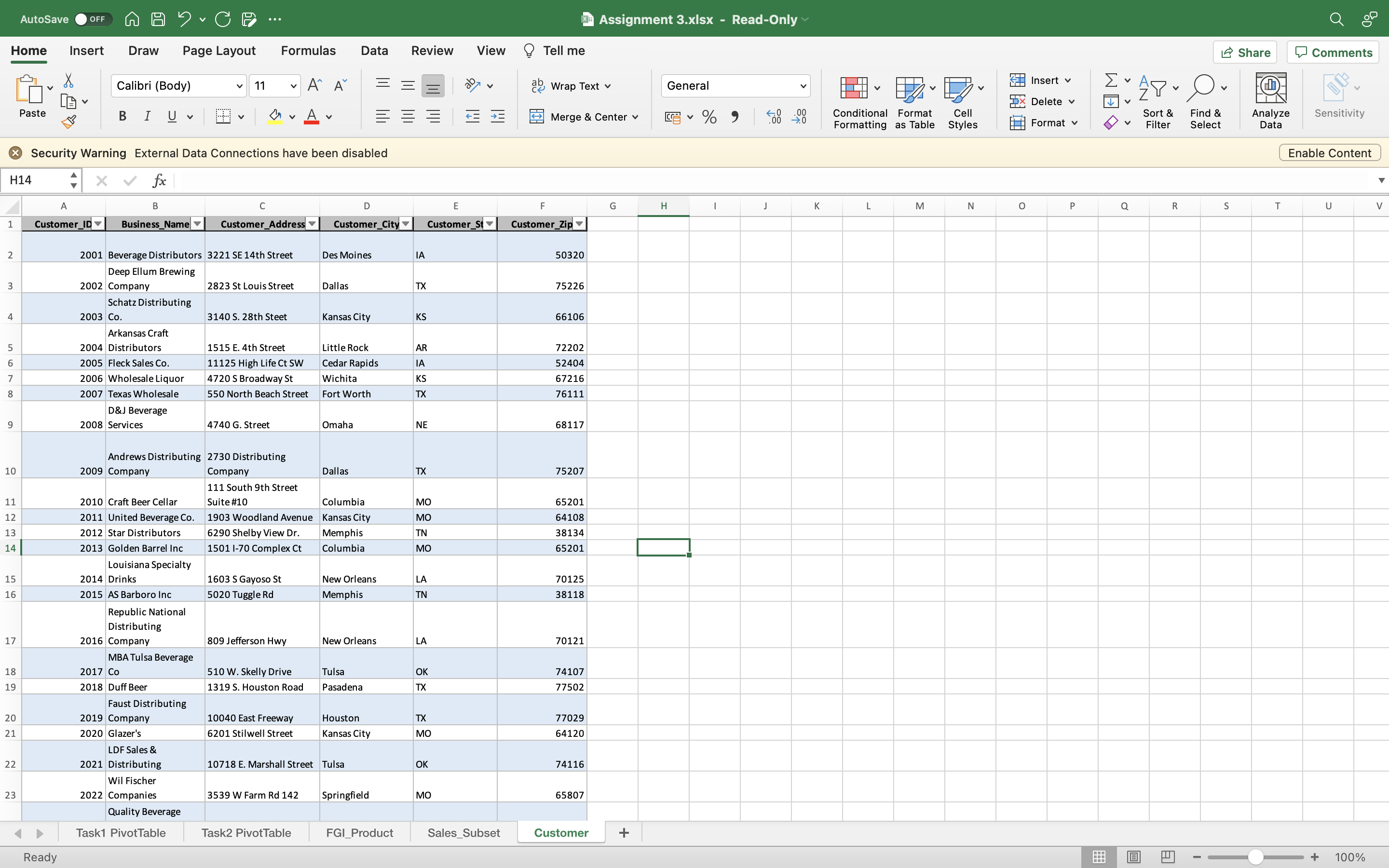
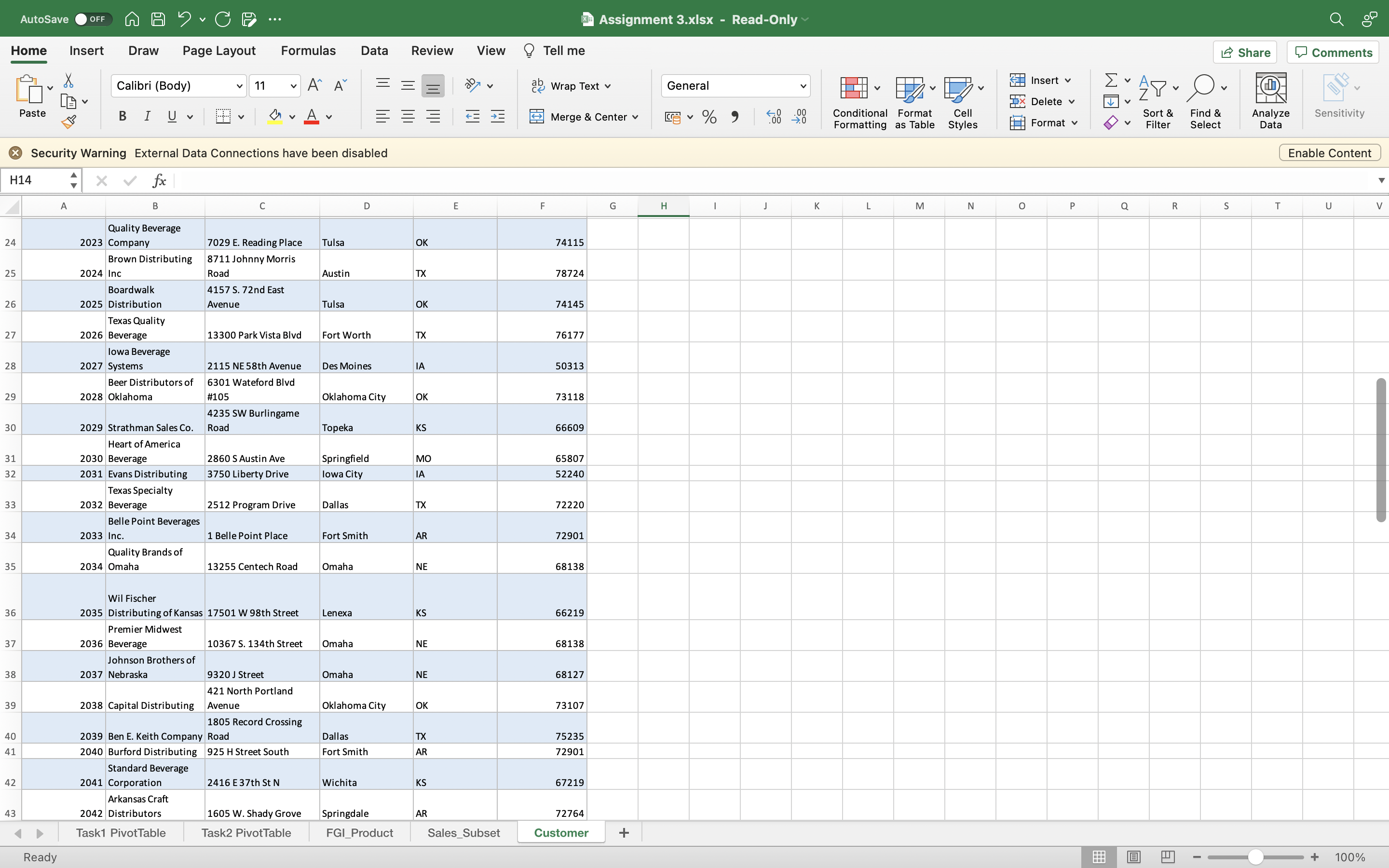
ACBZ420 Accounting Information Systems, Semester 2 2022. Assignment 3: Dashboard Design and Financial Modelling Due Date: Week 11. Friday 14 October 2022. 11:55pm (evening) AEST Weighting/Value: 20% Details of Task: This individual assignment assesses your ability to: (1) design a dashboard using Pivot Table and Pivot Chart to be used as part of management reporting systems. and (2) conduct Financial analysis using Excel spreadsheet. Release date: Week 9 Word limit: Equivalent to 1200 words Criteria for marking: Marks will be allocated based on the accuracy of your answers. screenshots and the dashboard design. Learning goals assessed: The assignment is designed to examine learning objectives 1, 3 & 4. Submission: Moodle Dropbox. Penalties for late submission: As per University guidelines. Note: The Assignment Coversheet is generated when you submit the assignment in Moodle. Ensure that you have read and understood the Monash Student Academic Integrity policy, and that the work you are submitting is not a result of plagiarism or collusion. Submission requirements: In a Microsoft Word document, write your answers to the questions (Q1425) in this assignment. and include the screenshots as instructed. Note that the word limit is word equivalent to the number of hours expected from you in completing this task. not a limit on the number of words in your submission. Please submit all documents (.docx and .xlsx) used to complete the tasks. Incomplete submission (missing file) will incur penalty. Name your file using the following format: YourLastname_YourFirstname_A3.docx and YourLastname_YourFirstname_A3.xlsx Instruction Create a Dashboard using Pivot Table and Pivot Chart in Microsoft Excel. following the instructions below. Write the answers to the five questions on Microsoft Word. including the screenshots when instructed. To create a screenshot in Windows. use the screen capture button. In Mac. use Control+Command+Shift+4. Penalty A penalty reduction of up to 2 grades will be imposed to the submitted work when the Excel spreadsheet is not submitted (2 grade penalty) or when the submitted spreadsheet is not demonstrating the derivation of the presented solution (1 grade penalty). Likewise. a penalty of one grade will be imposed if screenshot is missing. 80. please ensure that you include the screenshots from your Excel file to the Word document. ACB2420 Accounting Information Systems, Semester 2 2022. ACB2420 Accounting Information Systems, Semester 2 2022. 1. Spend a few minutes filtering the data with the slicers. Name three important insights that Background were easy to identify through this visualization. Slainte' is a hypothetical brewery that is undergoing major expansion. Slainte sells six different products. The brewery plans to expand its product distribution from one state to nine other states. The does the data visualization and the interactivity of the slicer provide your audience Business Manager would like to perform a data analysis using the transaction records to identify areas that the original Pivot Table does not? of successes, as well as areas of improvements. TASK 2: VISUALISING THE PIVOT TABLE WITH CONDITIONAL FORMATTING AND SPARKLINES Tasks Conditional formatting and sparklines are quick ways to visualize and compare data and trends when a Use the data file "Assignment3.xIsx" to carry out the following tasks: Creating a PivotChart and full-fledge chart is not necessary. Visualising the PivotTable with Conditional Formatting and Sparklines. Your work (submitted in Word 9. To quickly visualize how each product's total quantity sold over time compares across all six of Slainte's projects, we can apply document) should include the answers to Q1 to Q5 and 3 screenshots (from Excel). conditional formatting to the Grand Total column. Select the data in the Grand Total column of your PivotTable, and navigate to the Home tab on the ribbon. TASK 1: CREATING A PIVOT CHART B C D E 1 Sum of Sales_Order_Quantity_Sold Column Labels -Y Open Assignment3.xIsx. Start working with the "Sales Subset" worksheet. You will find a Table with multiple 2 Row Labels April February January March Grand Total columns in this worksheet. Create a Pivot Table (in a new sheet), then a Pivot Chart using the data in this Table. 3 Imperial IPA 17 23 2 42 4 Imperial Stout 36 21 61 42 166 Hint: You will need to select 3 items (Product_Code, Sales_Order_Date and Sales_Order_Quantity_Sold) in the 5 IPA 34 35 36 66 171 field name window and move it into the windows underneath (Rows, Columns and Values). Once organised, you 6 Pale Ale 18 A 27 32 81 can rename the Row Labels with "Product Description" and the decode the Product Code (2001 to 2006) with the Stout 16 33 65 4 118 8 Wheat 11 21 54 861 name of the product (using the FGI_Product worksheet). When done, execute the instructions below to create 9 Grand Total 121 110 233 200 664 the Pivot Chart. Source: Microsoft Excel for Mac 2020 1. Ensuring that the active cell in your workbook is somewhere in the PivotTable, navigate to the Analyze tab in the ribbon. 2. If you are working with a PC, you should see a button for PivotChart. If you are working with a Mac, you can insert a regular 10. From the Home tab, select the Conditional Formatting button, and a menu with the different types of formatting available chart from the Insert tab on the ribbon. Some of the functionality of this lab will be limited on a Mac, so you may opt to use a will appear. virtual PC lab environment to complete this lab. 11. Select Data Bars and pick the first option for blue gradient fill bars. 3. Once you click into PivotChart, a window for Insert Chart appears, along with a list of options for how you can visualize 12. This conditional formatting is helpful because it allows us to compare grand totals of each product. However, if we would like your PivotTable. It defaults to column chart. Another good option is the bar chart, which displays your data in horizontal bars to see how each product's month-over-month sales compare to one another, we can display mini line charts next to each row instead of columns. Create either a bar chart or a column chart by selecting the chart you prefer and clicking OK. with a sparkline. To do so, select all of the "meat" of your PivotTable-that is, don't select any of the product labels (such as Imperial IPA), month labels, or grand totals. 4. Take a screenshot that shows the PivotTable and the PivotChart (label it: Screenshot 1) C D E 5. The advantage of working with PivotCharts over regular charts is that you can slice and filter your data in the 1 Sum of Sales_Order_Quantity_Sold Column Labels -Y PivotTable and the PivotChart at the same time. If you are presenting your findings to a live audience and you anticipate N N Row Label April February January March Grand Total questions about specific months or specific products, using Excel's slicer tool is a great way to filter your data in a way that is Imperial IP 17 23 2 42 interactive and transparent. On the Analyze tab on the ribbon, you can select Insert Slicer. 4 Imperial Stout 36 27 61 42 166 6. In the window that pops up, select Product Description. This will create an interactive filter so that you can drill down into 5 34 35 36 66 171 18 4 27 81 different product descriptions as they perform over the months. 5 Pale Ale 32 7 Stout 16 33 65 118 7. Create a second slicer for Sales_Order_Date (Month). 8 Wheat 11 21 86 9 Grand Total 121 110 233 200 664 Source: Microsoft Excel for Mac 2020 8. Take a screenshot that includes the PivotChart, PivotTable, and both slicers (label it: Screenshot 2)ACB2420 Accounting Information Systems, Semester 2 2022. ACB2420 Accounting Information Systems, Semester 2 2022. 13. Navigate to the Insert tab on the ribbon, and select Line in the Sparklines category. 14. A window will appear specifying the data range you just selected and awaiting input for the Location Range. We'd like to see 25. In a new worksheet, perform a profitability analysis indicating the monthly sales ($) and the trend lines to the immediate right of our PivotTable, so you can select the cells in the first empty column after your Grand gross profit percentage for November 2019 to April 2020. Identify the most profitable product Totals. during this period and present an Excel chart to display the performance of the superior Sum of Sales_Order_Quantity_Sold Column Labels LY product. (You may choose which accounting metric(s) to present in the chart to demonstrate Row Labels April February January March Grand Total the performance.) Imperial IPA 17 23 2 Imperial Stout 36 27 61 42 166 |IPA 34 35 36 66 171 Pale Ale 18 4 27 32 The formula to calculate Gross Margin is as follows: 81 Stout 16 65 118 Gross Margin = Revenue - Cost of Goods Sold 33 Wheat 11 21 54 86 The formula to calculate gross margin as a percentage is Grand Total 121 110 233 200 664 Gross Margin % = [(Total Revenue - Cost of Goods Sold)/Total Revenue] x 100% Source: Microsoft Excel for Mac 2020 A 15. Click OK, and your sparklines will be created. 1 Product_Code Product_Description COGS 16. You will notice that there are gaps in the lines, though. If you'd rather see a continuous line to represent zero values for the N 200 Pale Ale $55 plank cells, you can change this option. Ensure that one of the cells with the sparkline in it is active, and navigate to the 3 2002 Imperial IPA $70 Sparkline Tools tab on the ribbon. 4 200 IPA $60 17. Click the bottom half of the Edit Data button to make a menu appear. 5 2004 Imperial Stout $65 18. From the menu, select Hidden & Empty Cells... 6 2005 Stou $50 19. Select the option to show empty cells as zero, and click OK. 7 2006 Wheat $55 20. Take a screenshot to show the conditional formatting and the sparklines (label it: Screenshot 3) Q3. When do you think a sparkline and/or conditional formatting would be preferable over creating a Pivot Chart? Q4. What other visualizations would be useful to interpret this data? If you were to create a report to be run smoothly, what are two visualizations that should be included? (PTO)AutoSave OFF A ACE... 3 Assignment 3.xIsx - Read-Only Home Insert Draw Page Layout Formulas Data Review View Tell me Share Comments Calibri (Body) 11 AA = ap Wrap Text v General Insert v Ex AY- O. Ex Delete v v Z Paste BIUV MvAv E Merge & Center v [ ~ % 9 00 20 Conditional Format Cell Sort & Find & Analyze Sensitivity Formatting as Table Styles Format v Filter Select Data Security Warning External Data Connections have been disabled Enable Content C34 fx A B C D E F G H J K L M N O P Q R S T W N Row Labels Sum of Sales_Order_Quantity_Sold 4 Imperial IPA 61 Imperial Stout 258 6 IPA 235 7 Pale Ale 116 8 Stout 190 9 Wheat 119 10 Grand Total 979 11 12 13 14 15 16 17 18 19 20 34 35 36 37 38 39 40 42 Task1 PivotTable Task2 PivotTable FGI_Product Sales_Subset Customer + Ready + 100%AutoSave O OFF A AGE ... 3 Assignment 3.xIsx - Read-Only Home Insert Draw Page Layout Formulas Data Review View Tell me Share Comments Calibri (Body) 11 AA ap Wrap Text v General Insert v Ex AY- O. Ex Delete v v Z Paste BIUV MvAv E E Merge & Center v ~ % 9 00 20 Conditional Format Cell Sort & Find & Analyze Sensitivity Formatting as Table Styles Format v Filter Select Data Security Warning External Data Connections have been disabled Enable Content C14 fx B C D E F G H J K L M N P Q R S T U V W Sum of Sales_Order_Quantity_Sold Column Labels 2 Row Labels April February January March Grand Total 3 Imperial IPA 17 23 4 Imperial Stout 36 61 166 5 IPA 34 36 171 6 Pale Ale 18 27 32 81 7 Stout 16 65 4 118 8 Wheat 21 54 86 9 Grand Total 121 110 233 200 664 10 11 12 13 14 15 16 17 18 19 20 28 33 34 35 36 37 38 39 40 42 Task1 PivotTable Task2 PivotTable FGI_Product Sales_Subset Customer + Ready + 100%AutoSave O OFF A A . G F ... Assignment 3.xlsx - Read-Only Home Insert Draw Page Layout Formulas Data Review View Table Tell me Share Comments Calibri 11 AA ab Wrap Text v Insert v = General Ex AY- O. Ex Delete v v Z Paste BIUV MvAv E E Merge & Center ~ % 9 00 20 Conditional Format Cell Sort & Find & Analyze Sensitivity Formatting as Table Styles Format v Filter Select Data Security Warning External Data Connections have been disabled Enable Content FGI_Prod... 4 X fx IPA C D E F G H I J K L M N P Q R S T U V W Product_Codi |Product_Description |Product_Sale_Price 2001 Pale Ale 95 2002 Imperial IPA 120 4 2003 IPA 100 5 2004 Imperial Stout 105 6 2005 Stout 85 7 2006 Wheat 90. 6 00 10 11 36 37 38 39 40 41 Task1 PivotTable Task2 PivotTable FGI_Product Sales_Subset Customer + Ready Average: 1051.333333 Count: 18 Sum: 12616 + 100%AutoSave OFF A ACP ... Assignment 3.xIsx - Read-Only Home Insert Draw Page Layout Formulas Data Review View Table Tell me Share Comments Insert v Calibri 11 AA ab Wrap Text v General Ex AY- O. Ex Delete v Z Sort & Find & Analyze Sensitivity Paste BIUV MvAv E Merge & Center v 00 80 Conditional Format Cell Formatting as Table Styles Format v Filter Select Data Security Warning External Data Connections have been disabled Enable Content G11 4 X V fx 100 A C D E G H I J K L M N 0 P Q R S T Sales_Order_In Sales_Order_Date sales_Employe Customer_ID Product_Code Sales_Order_Quantity_S| duct_Sal rice 20001 1/2019 1006 2056 2001 10 95 AWN 20003 1/11/2019 1006 2011 200 8 90 20005 1/11/2019 1006 2012 2006 9 90 20005 1/11/2019 1006 012 2001 8 95 20009 2/11/2019 1006 005 2004 3 105 20012 4/11/2019 1006 2009 2005 1 85 20013 4/11/2019 1007 2038 2003 2 100 20013 4/11/2019 1007 038 2002 4 120 20017 7/11/201 1006 2043 2001 1 95 20020 7/11/2019 1006 2032 2003 6 100 20023 8/11/2019 1007 2052 2005 2 85 20024 8/11/2019 1007 033 2004 11 105 20031 12/11/2019 1006 2022 2002 4 120 20033 12/11/2015 .007 2013 2003 1 100 20037 13/11/2019 1007 054 2004 w w 20037 13/11/2019 1007 2054 2005 85 20040 14/11/2019 1007 2037 200 2 100 20043 16/11/2019 1006 043 2005 12 20053 20/11/2019 1006 2035 2004 105 20055 20/11/2019 1007 039 2004 11 105 20056 21/11/2019 1006 2021 2003 8 100 20059 22/11/2019 1006 060 2005 6 85 20062 22/11/2019 1007 2001 2004 12 105 20063 22/11/2019 1006 2034 2003 4 100 20068 24/11/2019 1007 052 2004 9 105 20080 29/11/2019 1007 021 2001 11 95 28 20086 30/11/2019 1006 035 2005 11 85 29 20089 1/12/2019 1007 038 2005 10 85 30 20090 1/12/2019 1006 012 2002 10 120 20093 2/12/2019 1007 2058 2002 120 20097 4/12/2019 1007 2014 2003 100 0098 4/12/2019 1007 2037 2003 100 20103 5/12/2019 1006 060 2003 100 20106 7/12/2019 1006 2048 2004 1 105 36 20120 12/12/2019 1006 2031 2005 10 85 20124 15/12/2019 1007 2059 2004 11 105 38 20126 16/12/2019 1006 2048 2004 6 105 39 2012 16/12/2019 1006 2048 2005 9 85 40 20137 18/12/2019 1006 2056 2003 10 100 41 20138 19/12/2019 1007 041 2006 4 90 42 20140 1006 5 20/12/2019 2002 2001 95 Task1 PivotTable Task2 PivotTable FGI_Product Sales_Subset Customer + + 100% ReadyAutoSave OFF WHY CE ... Assignment 3.xIsx - Read-Only Home Insert Draw Page Layout Formulas Data Review View Table Tell me Share Comments Insert v Calibri v 11 AA - ap Wrap Text General O. Ex Delete v MvAV = Merge & Center [~ % 9 Conditional Format Cell Sort & Find & Analyze Sensitivity Paste BIUV - v Formatting as Table Styles Format Filter Select Data Enable Content x Security Warning External Data Connections have been disabled G11 X fx 105 Sales_Order_Quantity_S Produc H I K L M N 0 P Q R S T Sales_Order_ID Sales_Order_Date |Sales_Employ |Customer_ID |Product_Code 43 20155 23/12/2019 1006 2056 2003 8 100 44 20161 25/12/2019 1007 2019 2006 90 45 20163 25/12/2019 1006 2007 2003 3 100 20168 27/12/2019 1007 2001 2005 8 85 20179 30/12/2019 006 2036 2004 6 105 48 20183 1/1/2020 1006 2034 2002 10 120 20183 1/1/2020 1006 2034 200 7 95 20192 6/1/2020 1007 2061 2004 12 105 20199 7/1/2020 1007 2008 2005 8 85 20200 7/1/2020 1007 2043 2003 12 100 2020 7/1/2020 1007 043 2004 10 105 20202 8/1/2020 1006 2035 2005 7 85 2021 10/1/2020 1007 2013 2006 12 20211 10/1/202 1007 2013 2005 12 1007 11 100 20217 12/1/2020 2048 2003 :0218 12/1/2020 1007 2026 2004 105 20223 13/1/202 1006 2022 2001 95 20224 13/1/2020 1006 2007 2001 20227 14/1/2020 1006 2028 2001 20229 14/1/2020 1006 2019 2001 20230 15/1/2020 1006 2022 2002 FU DOWN VOI CO N H H A :0233 16/1/2020 1006 2006 2003 100 20241 19/1/2020 1007 2011 2004 105 20242 19/1/2020 1006 2061 2004 105 20249 22/1/2020 1006 2053 2004 105 20250 22/1/2020 1006 2010 2005 20251 22/1/2020 1007 010 2004 105 20253 22/1/2020 1007 2011 2005 10 20256 24/1/2020 1006 2034 2004 105 20261 25/1/2020 1006 2057 200 100 20262 26/1/2020 1007 2051 2005 12 85 20265 27/1/2020 1006 2023 2004 105 2026 27/1/2020 1006 022 2004 105 20271 28/1/2020 1007 2060 2005 11 85 20277 29/1/202 1006 2017 2006 1 90 20280 30/1/202 1006 2040 2006 4 90 1006 7 0280 30/1/202 2040 2001 95 20282 31/1/2020 1006 2050 2002 120 20283 31/1/2020 1007 2037 200 4 90 20285 1/2/2020 1007 050 2003 100 83 20291 4/2/202 007 2008 2005 85 84 3 85 0305 10/2/2020 1007 2021 2005 + D Task1 PivotTable Task2 PivotTable FGI_Product Sales_Subset Customer + 100% ReadyAutoSave O OFF A A . G E ... Assignment 3.xlsx - Read-Only View Table Tell me Share Comments Home Insert Draw Page Layout Formulas Data Review Insert v Calibri v 11 AA ab Wrap Text v General Ex AP - O. Ex Delete v Conditional Format Cell Sort & Find & Analyze Sensitivity Paste B IUVV E Merge & Center 08 20 Formatting as Table Styles Format Filter Select Data Enable Content Security Warning External Data Connections have been disabled G11 X fx 105 1 J K L M N P Q R S Sales_Order_ID Sales_Order_Date |Sales_Employ |Customer_ID |Product_Code H T Sales_Order_Quantity_S Produc 85 20305 10/2/2020 1007 2021 2001 95 105 86 20305 10/2/2020 1007 2021 2004 87 20307 11/2/2020 1007 2027 2004 105 88 20307 11/2/2020 1007 2027 2005 85 20308 11/2/2020 1006 2004 2004 105 89 100 90 20308 11/2/2020 1006 2004 2003 11/2/2020 1007 2002 2004 2 105 20310 92 20312 12/2/2020 1006 2021 2003 4 100 2 105 0314 13/2/2020 1007 2046 2004 20325 15/2/2020 1006 2058 200 7 100 17/2/2020 11 90 20328 1007 2037 2006 2013 2005 6 85 96 20338 22/2/2020 1006 97 20357 1006 2045 2005 8 85 27/2/2020 1007 2047 2003 11 100 98 20368 29/2/2020 99 20375 2/3/2020 1007 2029 2006 11/ 90 7 95 100 20378 3/3/2020 1007 2040 2001 101 20379 3/3/2020 1006 2020 2001 102 20383 4/3/2020 1007 2001 2004 105 100 103 20384 4/3/2020 1007 2037 2003 20393 7/3/2020 1007 2013 2003 100 104 10 105 20403 9/3/2020 1006 2040 2004 9/3/2020 1006 2024 2003 100 106 20404 107 20404 9/3/2020 1006 2024 2006 108 20406 10/3/2020 1007 2017 2005 85 10/3/2020 1006 2044 2004 105 109 20407 90 110 2040 10/3/2020 1006 2044 2006 2 100 111 20416 13/3/2020 1006 2040 2003 12 112 20418 14/3/2020 1006 2016 2006 90 16/3/2020 1006 50 2004 10 113 20424 105 114 20438 18/3/2020 1007 2028 2006 4 90 LOO 20439 1007 2056 2003 1 115 19/3/2020 116 20440 19/3/2020 1007 2039 2001 95 19/3/2020 1007 2062 2003 100 117 20441 2045 1007 046 2003 9 118 24/3/2020 100 119 20451 24/3/2020 1006 2008 2006 9 90 2 2045 24/3/2020 1006 120 120 2008 2002 1007 2022 2004 4 105 121 20452 25/3/2020 3 90 122 20453 25/3/2020 1007 2036 2006 20454 25/3/2020 2022 2003 1 123 1006 100 20457 26/3/2020 1006 2043 2001 10 95 124 2061 2003 11 1007 100 125 20458 26/3/2020 2050 2003 6 27/3/2020 1006 100 126 20460 Task2 PivotTable FGI_Product Sales_Subset Customer + D Task1 PivotTable + 100% ReadyN 0 Q T Sales_Order_Quantity_S Produc H I K L M P R S Sales_Order_ID Sales_Order_Date |Sales_Employ |Customer_ID| Product_Code 20461 27/3/2020 1007 2043 2004 105 127 105 128 20465 28/3/2020 1006 2029 2004 O W O OO N 2025 2003 100 129 20471 29/3/2020 1007 100 130 20491 7/4/2020 1006 2060 2003 20492 8/4/2020 1006 2057 2003 100 131 85 132 20494 8/4/2020 1006 2009 2005 105 20494 8/4/2020 1006 2009 2004 133 1A N 134 20495 8/4/2020 1007 2036 2005 85 105 135 20496 8/4/2020 2031 2004 85 10/4/2020 2062 2005 ONOUT 136 20503 1006 105 137 20503 10/4/2020 2062 2004 2025 2001 95 138 20513 13/4/2020 1007 139 20516 13/4/2020 1006 2039 2002 11 120 2049 2001 95 140 20518 14/4/2020 1007 2060 2003 11 100 141 20532 17/4/2020 1007 2045 2003 100 142 20535 19/4/2020 1007 143 20537 19/4/2020 1007 2009 2004 105 144 19/4/2020 1006 2053 2004 10 105 20539 100 145 20543 20/4/2020 1006 2016 2003 - W 100 146 20545 21/4/2020 1007 2043 2003 2042 2004 105 147 20559 25/4/2020 1007 2001 2002 120 148 20564 28/4/2020 1007 149 150 151 152 153 154 155 156 157 158 159 160 161 162 163 164 165 166 167 160 D Task1 PivotTable Task2 PivotTable FGI_Product Sales_Subset Customer + + 100% ReadyAutoSave O OFF A A . G P ... 3 Assignment 3.xIsx - Read-Only Home Insert Draw Page Layout Formulas Data Review View Tell me Share Comments Insert Calibri (Body) 11 AA = ab Wrap Text v General Ex AY- O. Ex Delete v v Z Analyze Sensitivity Paste BIUV MVAv E E Merge & Center v ~ % 9 Conditional Format Cell Sort & Find & Formatting as Table Styles Format v Filter Select Data Security Warning External Data Connections have been disabled Enable Content H14 X V fx A B C D E F G H I J K L M N P Q R S T U Customer_ID Business_Name Customer_Address Customer_City Customer_St Customer_Zip 2001 Beverage Distributors 3221 SE 14th Street Des Moines A 50320 Deep Ellum Brewing 3 2002 Company 2823 St Louis Street Dallas rx 75226 Schatz Distributing 2003 Co. 3140 S. 28th Steet Kansas City KS 66106 Arkansas Craft 2004 Distributors 1515 E. 4th Street Little Rock AR 72202 2005 Fleck Sales Co. 11125 High Life Ct SW Cedar Rapids IA 2404 2006 Wholesale Liquor 4720 S Broadway St Wichita KS 6721 2007 Texas Wholesale 550 North Beach Street Fort Worth TX 76111 D&J Beverage 2008 Services 4740 G. Street Omaha NE 68117 Andrews Distributing 2730 Distributing 10 2009 Company Company Dallas TX 75207 111 South 9th Street 11 2010 Craft Beer Cellar Suite #10 Columbia MO 65201 12 2011 United Beverage Co. 1903 Woodland Avenue Kansas City MC 54108 13 2012 Star Distributors 6290 Shelby View Dr. Memphis IN 30234 14 2013 Golden Barrel Inc 1501 1-70 Complex Ct Columbia MO 65201 Louisiana Specialty 15 2014 Drinks 1603 S Gayoso St New Orleans LA 70125 16 2015 AS Barboro Inc 5020 Tuggle Rd Memphis IN 38118 Republic National Distributing 17 2016 Company 809 Jefferson New Orleans LA 70121 MBA Tulsa Beverage 18 2017 Co 510 W. Skelly Drive Tulsa OK 74107 19 2018 Duff Beer 1319 S. Houston Road Pasadena TX 77502 Faust Distributing 20 2019 Company 10040 East Freeway Houston TX 77029 21 2020 Glazer's 6201 Stilwell Street Kansas City MO 64120 LDF Sales & 22 2021 Distributing 10718 E. Marshall Street Tulsa OK 74116 Wil Fischer 23 2022 Companies 3539 W Farm Rd 142 Springfield MO 65807 Quality Beverage Task1 PivotTable Task2 PivotTable FGI_Product Sales_Subset Customer + + 100% ReadyAutoSave O OFF A A . G E ... 3 Assignment 3.xIsx - Read-Only Home Insert Draw Page Layout Formulas Data Review View Tell me Share Comments Insert v Calibri (Body) 11 AA = ap Wrap Text v General Ex AY- O. Ex Delete v v Z Analyze Sensitivity Paste BIUV MVAv E Merge & Center v ~ % " 100 0 Conditional Format Cell Sort & Find & Formatting as Table Styles Format v Filter Select Data Security Warning External Data Connections have been disabled Enable Content H14 4 X V fx A C D E F G H I J K L M N 0 P Q R S T U B Quality Beverage 24 2023 Company 7029 E. Reading Place Tulsa OK 74115 Brown Distributing 8711 Johnny Morris 25 2024 Inc Road Austin TX 78724 Boardwalk 4157 S. 72nd East 26 2025 Distribution Avenue Tulsa OK 74145 Texas Quality 27 2026 Beverage 13300 Park Vista Blvd Fort Worth TX 76177 lowa Beverage 28 2027 Systems 2115 NE 58th Avenue Des Moines IA 50313 Beer Distributors of 6301 Wateford Blvd 2028 Oklahoma #10 Oklahoma City OK 73118 4235 SW Burlingame 30 2029 Strathman Sales Co. Road Topeka KS 66609 Heart of America 31 2030 Beverage 2860 S Austin Ave Springfield MO 65807 32 2031 Evans Distributing 3750 Liberty Drive lowa City IA 52240 Texas Specialty 33 2032 Beverage 2512 Program Drive Dallas TX 72220 Belle Point Beverages 34 2033 Inc. 1 Belle Point Place Fort Smith AR 72901 Quality Brands of 35 2034 Omaha 13255 Centech Road Omaha VE 6813 Wil Fischer 36 2035 Distributing of Kansas 17501 W 98th Street Lenexa (S 66219 Premier Midwest 37 2036 Beverage 10367 S. 134th Street Omaha NE 8138 Johnson Brothers of 38 2037 Nebraska 9320 J Street Omaha NE 68127 421 North Portland 39 2038 Capital Distributing Avenue Oklahoma City OK 3107 1805 Record Crossing 40 2039 Ben E. Keith Company Road Dallas TX 75235 41 2040 Burford Distributing 925 H Street South Fort Smith AR 72901 Standard Beverage 42 2041 Corporation 2416 E 37th St N Wichita KS 67219 Arkansas Craft 43 2042 Distributors 1605 W. Shady Grove Springdale AR 72764 Task1 PivotTable Task2 PivotTable FGI_Product Sales_Subset Customer + + 100% ReadyU F K L M N 0 Q R S T G H P A B D E 7777 Washington 44 2043 Silver Eagle Avenue Houston TX 77007 Grand Wholesale TX 79104 45 2044 Liquor Inc 09 S Grand St. Amarillo Premium Brands of 46 2045 NW Arkansas 1032 S. Razorback Road Fayetteville AR 72701 2046 Ben E. Keith Company 2300 N Lakeside Dr Amarillo TX 79108 47 City Wholesale 48 2047 Liquor Co 4340 Washington Ave New Orleans LA 70125 Reed Beverage 49 2048 Distributor 3333 SE 3rd Ave Amarillo TX 79104 50 2049 Doll Distributing Inc. 3501 23rd Avenue Council Bluffs IA 51501 Broadway Beer 2304 North Broadway 51 2050 Distributing Co Avenue Oklahoma City OK 73103 Capitol Wright South 3834 Promontory Point 2051 Austin Drive Austin TX 78744 52 53 2052 Sooner Beer Co th Tulsa Avenue Oklahoma City OK 73107 54 2053 Barn Spirits 3002 Chapel Hill Road Stillwater OK 74074 American Wholesale 3300 Pleasant Valley 55 2054 Distribution Lane Arlington TX 76015 North Kansas City 56 2055 Beverage Co. 203 E. 11th Avenue North Kansas City MO 64116 57 2056 General Distributors 800 EIndianapolis St. Wichita KS 67211 58 2057 BDT Beverage 2115 Spicer Cove #113 Memphis TN 38134 Standard Beverage 59 2058 Corporation 2300 Lakeview Road Lawrence KS 66049 60 2059 High Life Sales Co. 1900 W. 142nd Street Leawood KS 66224 Wholesale Beer 2060 Distributors 700 E. 9th Street #1J Little Rock AR 72202 61 62 2061 Nauser Beverage 6000 Paris Rd Columbia MO 65202 63 2062 De Nux Distributors 701 N. Broadway Street North Little Rock AR 72114 64 65 66 67 68 69 70 71 D Task1 PivotTable Task2 PivotTable FGI_Product Sales_Subset Customer + + 100% Ready