All must be done using R Complete these codes to achieve the desired outcome from this study answer guide, using my directory below to locate the file.

source("c:/users/olivier/Downloads/DBDA2Eprograms/DBDA2Eprograms/ Here is my R code for the two parts: #Part (a)

## Question 1

# Load necessary libraries library(rjags) library(coda)

# Load the data data

# Prepare data for JAGS jags_data

# Define the JAGS model model_string

# Run the JAGS model model

# Analyze the results summary(samples)

Part (b)

# Load the data data

# Explore the data str(data) summary(data)

# Visualize the total consumption ggplot(data, aes(x = Group, y = GrandTotal)) + geom_boxplot() + labs(title = "Total Food Consumption by Group", x = "Group", y = "Total Consumption (ml)") # Perform a t-test to compare the means of the two groups t_test_result

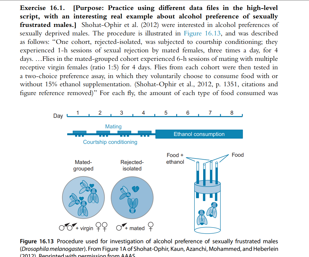
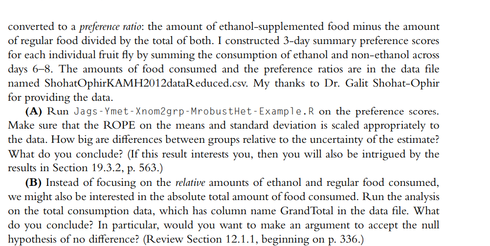
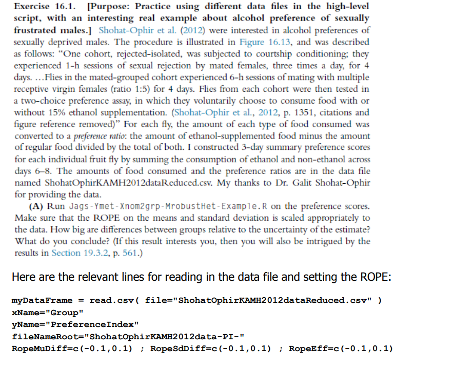
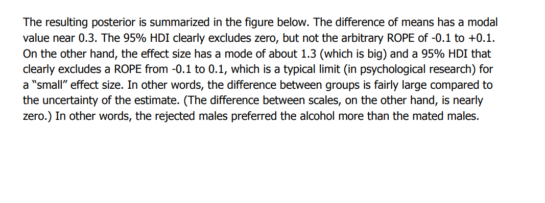
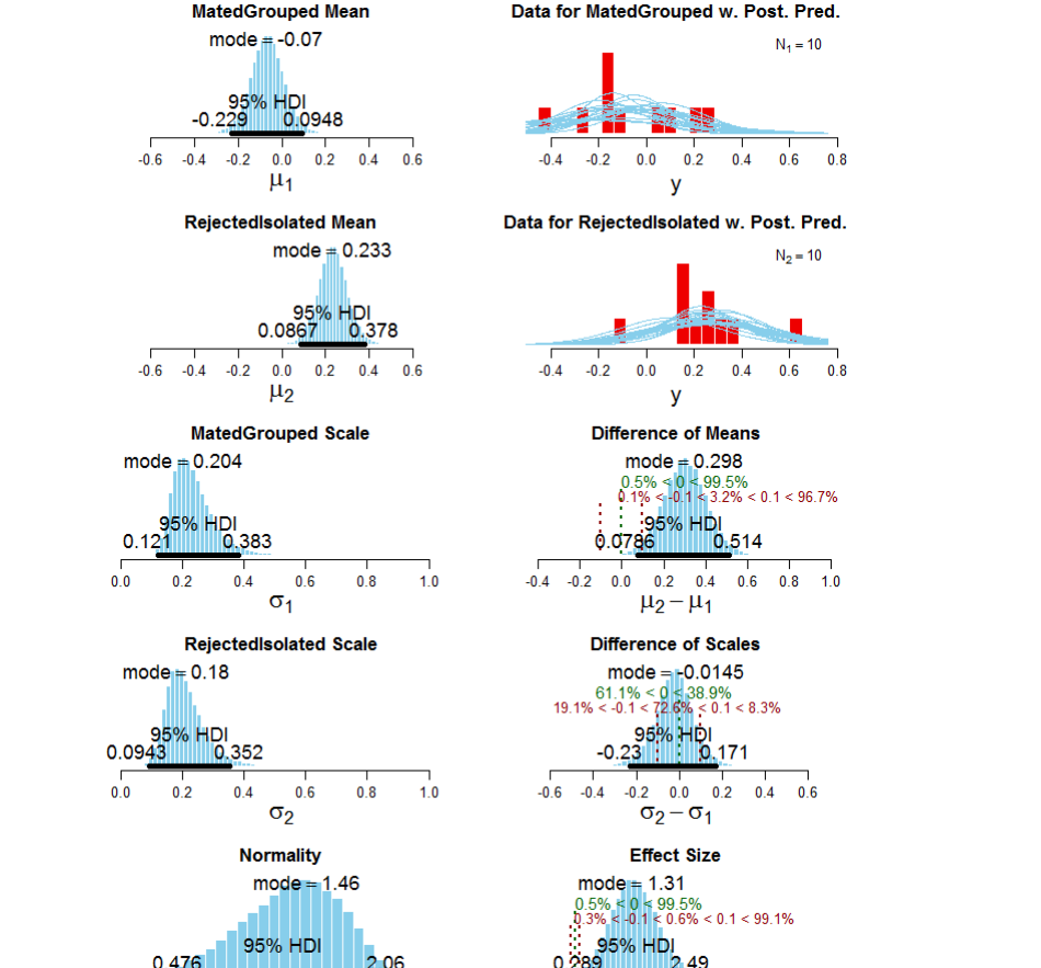
Exercise 16.1. [Purpose: Practice using different data files in the high-level script, with an interesting real example about alcohol preference of sexually frustrated males.] Shohat-Ophir et al. (2012) were interested in alcohol preferences of sexually deprived males. The procedure is illustrated in Figure 16.13, and was described as follows: "One cohort, rejected-isolated, was subjected to courtship conditioning; they experienced 1-h sessions of sexual rejection by mated females, three times a day, for 4 days. ...Flies in the mated-grouped cohort experienced 6-h sessions of mating with multiple receptive virgin females (ratio 1:5) for 4 days. Flies from each cohort were then tested in a two-choice preference assay, in which they voluntarily choose to consume food with or without 15% ethanol supplementation. (Shohat-Ophir et al., 2012, p. 1351, citations and figure reference removed)" For each fly, the amount of each type of food consumed was Day L 2 3 4 5 6 7 8 Mating Ethanol consumption Courtship conditioning Food + Food Mated- Rejected- ethanol grouped isolated O'O'+ virgin $8 + mated Figure 16.13 Procedure used for investigation of alcohol preference of sexually frustrated males (Drosophila melanogaster). From Figure 1A of Shohat-Ophir, Kaun, Azanchi, Mohammed, and Heberleinconverted to a preference ratio: the amount of ethanol-supplemented food minus the amount of regular food divided by the total of both. I constructed 3-day summary preference scores for each individual fruit fly by summing the consumption of ethanol and non-ethanol across days 6-8. The amounts of food consumed and the preference ratios are in the data file named ShohatOphirKAMH2012dataReduced.csv. My thanks to Dr. Galit Shohat-Ophir for providing the data. (A) Run Jags-Ymet-Xnom2grp-MrobustHet-Example.R on the preference scores. Make sure that the ROPE on the means and standard deviation is scaled appropriately to the data. How big are differences between groups relative to the uncertainty of the estimate? What do you conclude? (If this result interests you, then you will also be intrigued by the results in Section 19.3.2, p. 563.) (B) Instead of focusing on the relative amounts of ethanol and regular food consumed, we might also be interested in the absolute total amount of food consumed. Run the analysis on the total consumption data, which has column name GrandTotal in the data file. What do you conclude? In particular, would you want to make an argument to accept the null hypothesis of no difference? (Review Section 12.1.1, beginning on p. 336.) Exercise 16.1. [Purpose: Practice using different data files in the high-level script, with an interesting real example about alcohol preference of sexually frustrated males.] Shohat-Ophir et al. (2012) were interested in alcohol preferences of sexually deprived males. The procedure is illustrated in Figure 16.13, and was described as follows: "One cohort, rejected-isolated, was subjected to courtship conditioning; they experienced 1-h sessions of sexual rejection by mated females, three times a day, for 4 days. ...Flies in the mated-grouped cohort experienced 6-h sessions of mating with multiple receptive virgin females (ratio 1:5) for 4 days. Flies from each cohort were then tested in a two-choice preference assay, in which they voluntarily choose to consume food with or without 15% ethanol supplementation. (Shohat-Ophir et al., 2012, p. 1351, citations and figure reference removed)" For each fly, the amount of each type of food consumed was converted to a preference ratio: the amount of ethanol-supplemented food minus the amount of regular food divided by the total of both. I constructed 3-day summary preference scores for each individual fruit fly by summing the consumption of ethanol and non-ethanol across days 6-8. The amounts of food consumed and the preference ratios are in the data file named ShohatOphirKAMH2012dataReduced.csv. My thanks to Dr. Galit Shohat-Ophir for providing the data. (A) Run Jags -Ymet - Xnom2grp-MrobustHet - Example. R on the preference scores. Make sure that the ROPE on the means and standard deviation is scaled appropriately to the data. How big are differences between groups relative to the uncertainty of the estimate? What do you conclude? (If this result interests you, then you will also be intrigued by the results in Section 19.3.2, p. 561.) Here are the relevant lines for reading in the data file and setting the ROPE: myDataFrame = read. csv( file="ShohatOphirKAMH2012dataReduced. csv" ) xName="Group" yName="PreferenceIndex" fileNameRoot="ShohatOphirKAMH2012data-PI-" RopeMuDiff=c (-0. 1, 0.1) ; RopeSdDiff=c (-0.1,0.1) ; RopeEff=c (-0.1,0.1)The resulting posterior is summarized in the figure below. The difference of means has a modal value near 0.3. The 95% HDI clearly excludes zero, but not the arbitrary ROPE of -0.1 to +0.1. On the other hand, the effect size has a mode of about 1.3 (which is big) and a 95% HDI that clearly excludes a ROPE from -0.1 to 0.1, which is a typical limit (in psychological research) for a \"small\" effect size. In other words, the difference between groups is fairly large compared to the uncertainty of the estimate. (The difference between scales, on the other hand, is nearly zero.) In other words, the rejected males preferred the alcohol more than the mated males. MatedGrouped Mean Data for MatedGrouped w. Post. Pred. mode = -0.07 N1 = 10 95% HDI -0.229 0.0948 0.6 -0.4 -0.2 0.0 0.2 0.4 0.6 -0.4 -0.2 0.0 0.2 0.4 0.6 0.8 H1 y Rejectedisolated Mean Data for Rejectedisolated w. Post. Pred. mode # 0.233 N2 - 10 95% HDI 0.0867 0.378 -0.6 -0.4 -0.2 0.0 0.2 0.4 0.6 -0.4 -0.2 0.0 0.2 0.4 0.6 0.8 H2 MatedGrouped Scale Difference of Means mode = 0.204 mode = 0.298 0.5% $ 0 -99.5% 0.1%