

Question: Create a Bank Reconciliation for Auto Salvage Co. In this exercise, you will create a bank reconciliation for Auto Salvage Co. for the month

![save the file in your Chapter 05 folder as: EA5-R1-BankRec-[YourName] 2. Enter](https://dsd5zvtm8ll6.cloudfront.net/si.experts.images/questions/2022/01/61eff0f4a99a2_1643114739935.jpg)
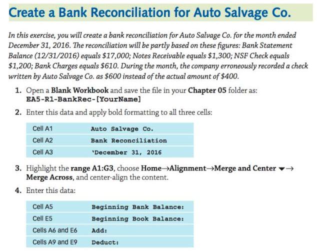
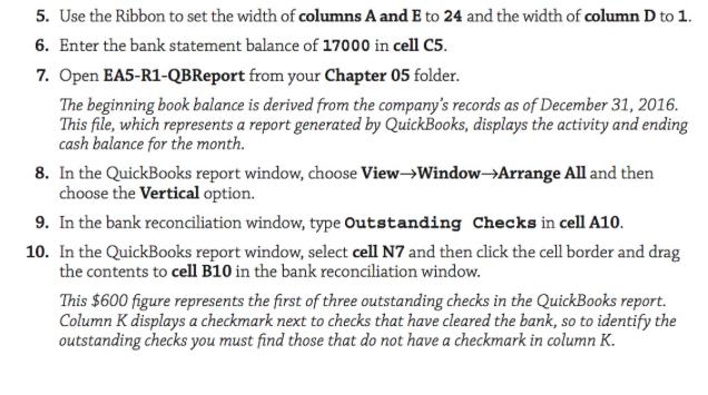
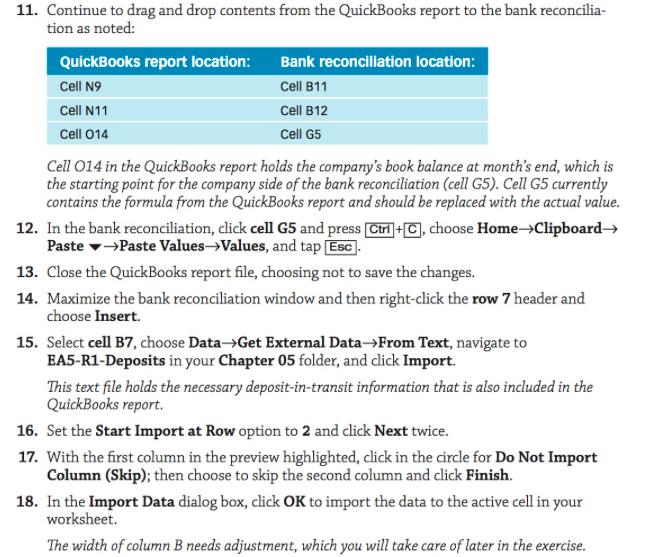
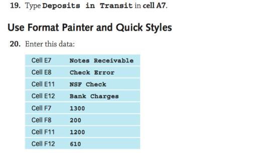
Create a Bank Reconciliation for Auto Salvage Co. In this exercise, you will create a bank reconciliation for Auto Salvage Co. for the month ended December 31, 2016. The reconciliation will be partly based on these figures: Bank Statement Balance (12/31/2016) equals $17,000; Notes Receivable equals $1,300; NSF Check equals $1,200; Bank Charges equals $610. During the month, the company erroneously recorded a check written by Auto Salvage Co. as $600 instead of the actual amount of $400. 1. Open a Blank Workbook and save the file in your Chapter 05 folder as: EA5-R1-BankRec-[YourName] 2. Enter this data and apply bold formatting to all three cells: Cell A1 Cell A2 Cell A3 Auto Salvage Co. Bank Reconciliation 'December 31, 2016 3. Highlight the range A1:G3, choose Home Alignment Merge and Center Merge Across, and center-align the content. 4. Enter this data: Cell A5 Cell E5 Cells A6 and E6 Cells A9 and E9 Beginning Bank Balance: Beginning Book Balance: Add: Deduct: 5. Use the Ribbon to set the width of columns A and E to 24 and the width of column D to 1. 6. Enter the bank statement balance of 17000 in cell C5. 7. Open EA5-R1-QBReport from your Chapter 05 folder. The beginning book balance is derived from the company's records as of December 31, 2016. This file, which represents a report generated by QuickBooks, displays the activity and ending cash balance for the month. 8. In the QuickBooks report window, choose View-Window-Arrange All and then choose the Vertical option. 9. In the bank reconciliation window, type Outstanding Checks in cell A10. 10. In the QuickBooks report window, select cell N7 and then click the cell border and drag the contents to cell B10 in the bank reconciliation window. This $600 figure represents the first of three outstanding checks in the QuickBooks report. Column K displays a checkmark next to checks that have cleared the bank, so to identify the outstanding checks you must find those that do not have a checkmark in column K. 11. Continue to drag and drop contents from the QuickBooks report to the bank reconcilia- tion as noted: QuickBooks report location: Cell N9 Cell N11 Cell 014 Bank reconciliation location: Cell B11 Cell B12 Cell G5 Cell 014 in the QuickBooks report holds the company's book balance at month's end, which is the starting point for the company side of the bank reconciliation (cell G5). Cell G5 currently contains the formula from the QuickBooks report and should be replaced with the actual value. 12. In the bank reconciliation, click cell G5 and press [Ctrl+C), choose HomeClipboard Paste Paste Values-Values, and tap [Esc]. 13. Close the QuickBooks report file, choosing not to save the changes. 14. Maximize the bank reconciliation window and then right-click the row 7 header and choose Insert. 15. Select cell B7, choose Data Get External Data From Text, navigate to EA5-R1-Deposits in your Chapter 05 folder, and click Import. This text file holds the necessary deposit-in-transit information that is also included in the QuickBooks report. 16. Set the Start Import at Row option to 2 and click Next twice. 17. With the first column in the preview highlighted, click in the circle for Do Not Import Column (Skip); then choose to skip the second column and click Finish. 18. In the Import Data dialog box, click OK to import the data to the active cell in your worksheet. The width of column B needs adjustment, which you will take care of later in the exercise. 19. Type Deposits in Transit in cell A7. Use Format Painter and Quick Styles 20. Enter this data: Cell E7 Cell E8 Cell E11 Cell E12 Cell F7 Cell F8 Cell F11 Cell F12 Notes Receivable Check Error NSF Check Bank Charges 1300 200 1200 610 21. Enter =Sum(B7:B8) in cell C8 and then use the Ribbon to copy cell C8 and paste to cells G8, C13, and G12. 22. Select cell C13, highlight B12 in the Formula Bar, click cell B11, and tap [Enter 23. Enter =Sum (C5:C8) in cell C9 and then use keyboard shortcuts to copy cell C9 and paste to cell G9. 24. Select cell C14, type =C9- and click cell C13, and tap [Enter]. Copy cell C14 and paste to cell G14 using the method of your choice. 25. With cell G14 selected, highlight G13 in the Formula Bar, click cell G12, and tap Enter 26. Enter Adjusted Bank Balance in cell A14 and Adjusted Book Balance in cell E14. 27. In cell C5, choose HomeNumber Accounting Number Format and then click Decrease Decimal twice. 28. Go to HomeClipboard and double-click Format Painter. 29. Click once on every cell and range in which numbers are displayed and then choose HomeClipboard Format Painter to turn off Format Painter. 30. Select the headers for columns B-C and columns F-G and then double-click between the columns F and G headers. 31. Apply a bottom border to cells C8, C13, G8, and G12; set a bottom double border to cell C14 and paint the formatting to cell G14. 32. Select cells A5, A14, E5, and E14 and then choose Home Styles Cell Styles Heading 4. Apply Conditional Formatting You want to be alerted if the bank balance drops below $20,000 at the end of any month so additional steps may be taken. You will now apply conditional formatting to set up the alert. 33. Select cell C5, choose Home Styles Conditional Formatting Manage Rules, and click the New Rule button. 34. Set up the rule as indicated: Rule type: Use a Formula to Determine Which Cells to Format Rule description: =$C$5
Step by Step Solution
3.49 Rating (176 Votes )
There are 3 Steps involved in it
Bank Reconciliation for Auto Salvage Co Month Ended December 31 2016 Open a Blank Workbook and save ... View full answer

Get step-by-step solutions from verified subject matter experts