ANSC $221$ HWEX$1$

Homework Exercise $-$ Excel Spreadsheet for Nutritional Calculations

Version $5,$ Update $11/11/19$

The purpose of this exercise is to learn some elementary things about use of Excel spreadsheets for making calculations, that can be very useful in nutrition. Many of you may already know all of these things and more $($and that's fine$),$ and others may have never used Excel, so this will be at a very simple level.

You are to make a spreadsheet that will make useful calculations. Print a copy of the spreadsheet to turn in $($so it should be arranged to nicely fit on one page$).$

Follow these directions:

In Cell A$1$ type ANSC $221$ Homework Excel$-1\{$YOUR NAME$\}$ and press Enter. $($Of course type your own name and not literally $"\{$YOUR NAME$\}"$

I will show you how to make a simple ration checking program that will multiply feed amounts times the nutrient content of feeds, and add up the results. List some feeds in rows $3$ through $10$ in column $1.$ Now copy those feed names to rows $13-20$ by doing the following. Highlight the feed names you typed in rows $3-10.$ Hit Control$-$C$.$ Place your cursor in cell A$13$ and left click the mouse. Press Control$-$V $($which pastes what you copied with Control$-$C$).$ Let's also copy those names to cells A$23$ to A$30.$ Press ESC $($escape$)$ to release the area you highlighted.

Let's format this so the feed names all sit in column A$.$ Move your cursor to the spot between the A and $B$ at the top of the spreadsheet cells. Left click, and when the cursor changes to a line with arrows to both sides, left$-$click again and drag the A$-$column wider so that the feed names all fit within column A$.$

Let's put labels above the columns: on row $2$ in column B enter AMOUNT, in C enter CP$,$ in D enter TDN$,$ in $E$ enter $CA,$ in $F$ enter $P.$ Of course you could do the same thing with other and more nutrients.

From data on nutrient content $($from somewhere$),$ enter the percentage of CP$,$ TDN$,$ Ca$,$ and $P$ for the feeds you chose. $($Leave the "Amount" column blank$).$

Next, we are going to want to multiply the feed amounts we specify by the DECIMAL values for the percentages we entered, or in other words, by those amounts divided by $100.$ Let's go to Cell C$13($for timothy hay on my sample page, CP column$)$ and write a formula that takes the value in cell C$3$ and divides it by $100.$ Start your formula by entering the $=$ sign. So in cell C$13$ enter $=$ then click on cell C$3,$ enter $"\frac{?}{?}"($for divide$)$ enter $100$ and then press the enter key. $($To multiply it would be the asterisk symbol, ${?}^{**})$

Now we could do that for every cell, but there is a much faster way. Click in cell C$13.$ Notice at the bottom right the box has a dense square. Move your cursor over it until it forms a $+.$ Click that square and drag right to copy the contents $($the formula$)$ to Cells D through F$.$ Alternatively, in Cell C$13$ we could have hit Control$-$C$,$ clicked in Cell D$13,$ dragged right to Cell F$13,$ released and pressed Control$-$V $($and it would do the same thing$).$ CTRL$-$C copies to your clipboard, and CTRL$-$V pastes from your clipboard.Note that to undo something you could click the circular arrow pointing left at the top, and to redo you could click the circular arrow to the right at the top of the page. Sometimes Excel is not set up with all the same icons in the same page, but that can be adjusted and they are commonly there.

Now let's copy those formulas down. Click in C$13$ and drag right to highlight C$13-$F$13.$ Release the click, and then hover over that dot in the lower right corner of the line around the cells highlighted, and then drag down to include row $20,$ then release. $($This could also be done with CTRL$-$C $-$ CTRL$-$V$.)$

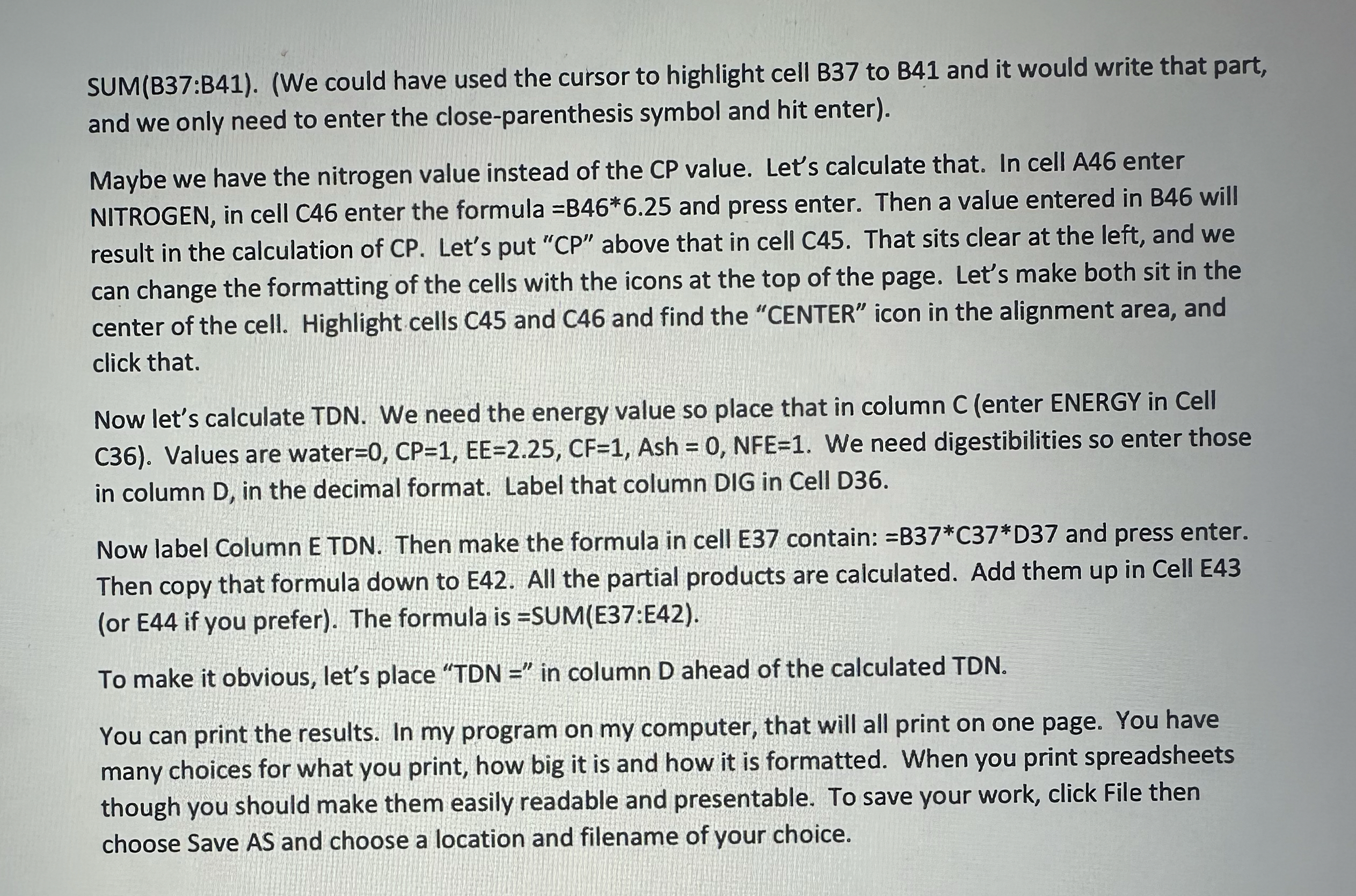
Now let's make our multiplications. First you may enter values for each feed amount in column B$,$ rows $23-30.$ These are the values you can change to get different results, so for now it isn't important what value you enter, BUT MAKE THEM DIFFERENT FROM THE EXAMPLE PAGE so it shows your sheet makes calculations. But we want EACH value $($in column B$)$ multiplied by the correct value in column C$.$ If you enter a formula in cell C$23$ as we did in cell C$13$ and then copy that, the program will automatically adjust the formula. We don't want it to change the formula, we want it to always use the value in column B$,$ so we are going to enter a $"$$$"$ sign in front of a cell reference to "root" it so that it doesn't change. In Cell C$23$ enter: $=$$$B{23}^{**}C13$ and press enter. The calculation is shown $($but the cell contains the formula$).$ Now we can copy the formula in Cell C$23$ to cells D$,$ E and F$.($Do that with the click, click the $+$ and drag, or use the CTRL$-$C$,$ CTRL$-$V method$).$ Then you can highlight all $4$ cells $($C$23-$F$23)$ and copy them down to row $30($by either method$).$

$($There is another