Answer if you can. Not forcing anyone.

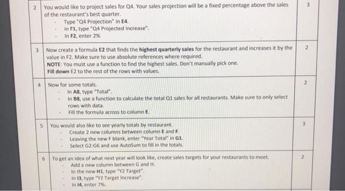
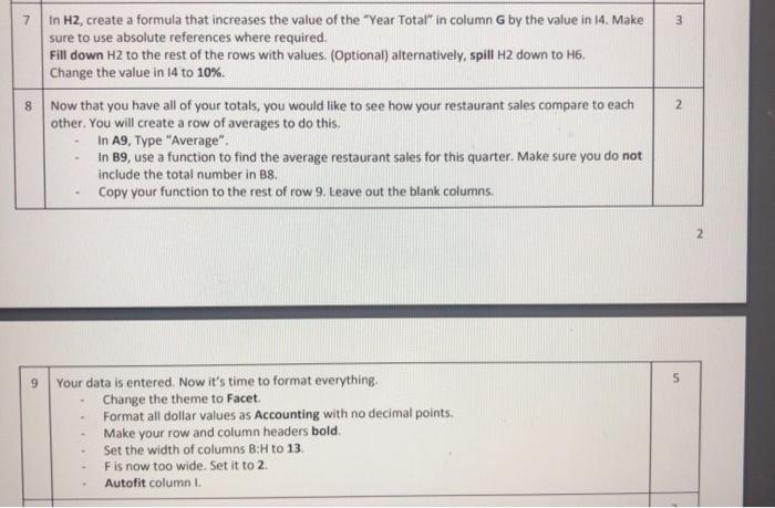
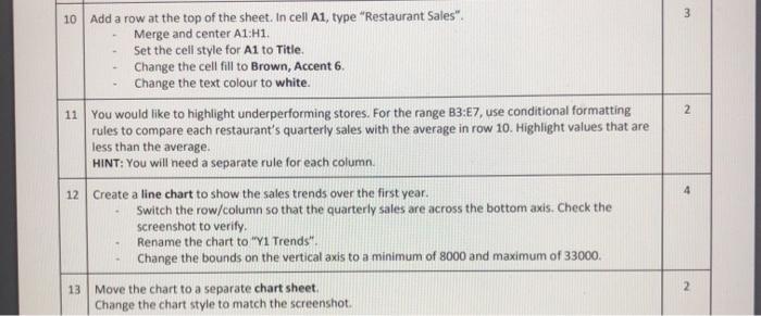
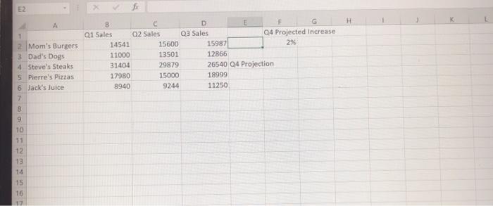
3 2 2 3 You would like to project sales for 04. Your sales projection will be a fixed percentage above the sales of the restaurant's best quarter. Type"Q4 Projection" in E4. In F1, type "Q4 Projected increase". In F2, enter 2% Now create a formula E2 that finds the highest quarterly sales for the restaurant and increases it by the value in F2. Make sure to use absolute references where required. NOTE: You must use a function to find the highest sales. Don't manually pick one. Fill down E2 to the rest of the rows with values. Now for some totals. In A8, type "Total" in B8, use a function to calculate the total Q1 sales for all restaurants. Make sure to only select rows with data Fill the formula across to column 2 5 3 You would also like to see yearly totals by restaurant Create 2 new columns between column E and F Leaving the new F blank, enter "Year Total" in 1 Select 62:66 and use AutoSum to fill in the totals. To get an idea of what next year will look like, create sales targets for your restaurants to meet. Add a new column between G and H. in the new H1, type "Y2 Target": In 13, type "Y2 Target Increase", In 14, enter 7% 2 7 3 8 In H2, create a formula that increases the value of the "Year Total" in column G by the value in 14. Make sure to use absolute references where required. Fill down H2 to the rest of the rows with values. (Optional) alternatively, spill H2 down to H6. Change the value in 14 to 10%. Now that you have all of your totals, you would like to see how your restaurant sales compare to each other. You will create a row of averages to do this. In A9, Type "Average". In B9, use a function to find the average restaurant sales for this quarter. Make sure you do not include the total number in B8. Copy your function to the rest of row 9. Leave out the blank columns 2 2 9 5 Your data is entered. Now it's time to format everything. Change the theme to Facet. Format all dollar values as Accounting with no decimal points. Make your row and column headers bold. Set the width of columns B:H to 13 Fis now too wide. Set it to 2. Autofit column 1 3 10 Add a row at the top of the sheet. In cell A1, type "Restaurant Sales". Merge and center A1:H1. Set the cell style for A1 to Title Change the cell fill to Brown, Accent 6. Change the text colour to white. 11 You would like to highlight underperforming stores. For the range B3:7, use conditional formatting rules to compare each restaurant's quarterly sales with the average in row 10. Highlight values that are less than the average. HINT: You will need a separate rule for each column. 2 4 12 Create a line chart to show the sales trends over the first year. Switch the row/column so that the quarterly sales are across the bottom axis. Check the screenshot to verify Rename the chart to "Y1 Trends". Change the bounds on the vertical axis to a minimum of 8000 and maximum of 33000 2 13 Move the chart to a separate chart sheet. Change the chart style to match the screenshot E2 H K B c D F G Q1 Sales 02 Sales Q3 Sales Q4 Projected Increase 14541 15600 159871 29 11000 13501 12866 31404 29879 26540 Q4 Projection 17980 15000 1.8999 8940 9244 11250 A 1 2 Mom's Burgers 3 Dad's Dogs 4 Steve's Steaks 5 Pierre's Pizzas 6 Jack's Juice 7 B 9 10 11 12 13 14 16 3 2 2 3 You would like to project sales for 04. Your sales projection will be a fixed percentage above the sales of the restaurant's best quarter. Type"Q4 Projection" in E4. In F1, type "Q4 Projected increase". In F2, enter 2% Now create a formula E2 that finds the highest quarterly sales for the restaurant and increases it by the value in F2. Make sure to use absolute references where required. NOTE: You must use a function to find the highest sales. Don't manually pick one. Fill down E2 to the rest of the rows with values. Now for some totals. In A8, type "Total" in B8, use a function to calculate the total Q1 sales for all restaurants. Make sure to only select rows with data Fill the formula across to column 2 5 3 You would also like to see yearly totals by restaurant Create 2 new columns between column E and F Leaving the new F blank, enter "Year Total" in 1 Select 62:66 and use AutoSum to fill in the totals. To get an idea of what next year will look like, create sales targets for your restaurants to meet. Add a new column between G and H. in the new H1, type "Y2 Target": In 13, type "Y2 Target Increase", In 14, enter 7% 2 7 3 8 In H2, create a formula that increases the value of the "Year Total" in column G by the value in 14. Make sure to use absolute references where required. Fill down H2 to the rest of the rows with values. (Optional) alternatively, spill H2 down to H6. Change the value in 14 to 10%. Now that you have all of your totals, you would like to see how your restaurant sales compare to each other. You will create a row of averages to do this. In A9, Type "Average". In B9, use a function to find the average restaurant sales for this quarter. Make sure you do not include the total number in B8. Copy your function to the rest of row 9. Leave out the blank columns 2 2 9 5 Your data is entered. Now it's time to format everything. Change the theme to Facet. Format all dollar values as Accounting with no decimal points. Make your row and column headers bold. Set the width of columns B:H to 13 Fis now too wide. Set it to 2. Autofit column 1 3 10 Add a row at the top of the sheet. In cell A1, type "Restaurant Sales". Merge and center A1:H1. Set the cell style for A1 to Title Change the cell fill to Brown, Accent 6. Change the text colour to white. 11 You would like to highlight underperforming stores. For the range B3:7, use conditional formatting rules to compare each restaurant's quarterly sales with the average in row 10. Highlight values that are less than the average. HINT: You will need a separate rule for each column. 2 4 12 Create a line chart to show the sales trends over the first year. Switch the row/column so that the quarterly sales are across the bottom axis. Check the screenshot to verify Rename the chart to "Y1 Trends". Change the bounds on the vertical axis to a minimum of 8000 and maximum of 33000 2 13 Move the chart to a separate chart sheet. Change the chart style to match the screenshot E2 H K B c D F G Q1 Sales 02 Sales Q3 Sales Q4 Projected Increase 14541 15600 159871 29 11000 13501 12866 31404 29879 26540 Q4 Projection 17980 15000 1.8999 8940 9244 11250 A 1 2 Mom's Burgers 3 Dad's Dogs 4 Steve's Steaks 5 Pierre's Pizzas 6 Jack's Juice 7 B 9 10 11 12 13 14 16