answer instructions 1-8 for a like please and thank you!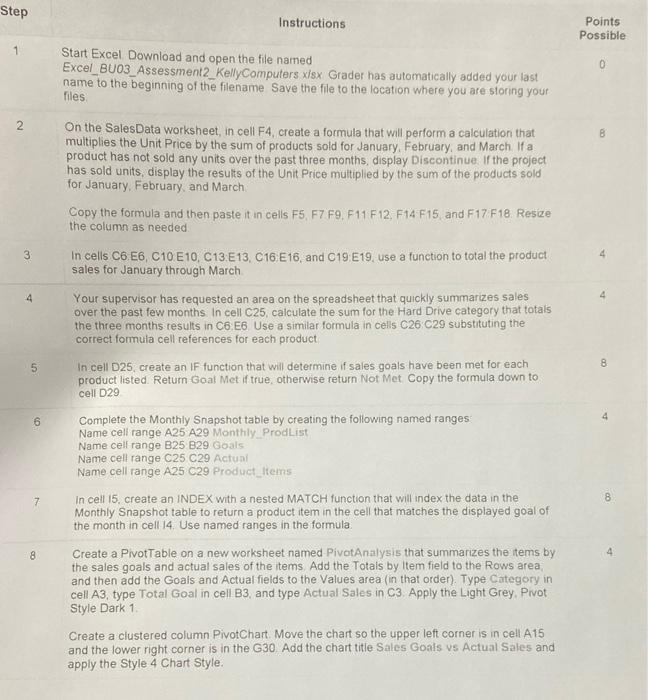

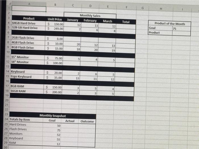
Step Instructions Points Possible 1 Start Excel Download and open the file named Excel_BU03_Assessment2_KellyComputers x/sx Grader has automatically added your last name to the beginning of the filename Save the file to the location where you are storing your 0 Tiles 2 B On the Sales Data worksheet, in cell F4 create a formula that will perform a calculation that multiplies the Unit Price by the sum of products sold for January, February, and March If a product has not sold any units over the past three months, display Discontinue. If the project has sold units, display the results of the Unit Price multiplied by the sum of the products sold for January, February, and March Copy the formula and then paste it in cells F5, F7 F9. F11 F12, F14 F15 and F17 F18 Resize the column as needed 3 4 4 8 5 6 4 In cells C6 E6, C10 E10, C13 E13, C16 E16, and C19 E19. use a function to total the product sales for January through March Your supervisor has requested an area on the spreadsheet that quickly summarizes sales over the past few months. In cell C25, calculate the sum for the Hard Drive category that totals the three months results in C6 E6 Use a similar formula in cells C26 C29 substituting the correct formula cell references for each product In cell D25, create an IF function that will determine if sales goals have been met for each product listed Return Goal Metif true, otherwise return Not Met Copy the formula down to cell D29 Complete the Monthly Snapshot table by creating the following named ranges Name cell range A25 A29 Monthly ProdList Name cell range B25 B29 Goals Name cell range C25 C29 Actual Name cell range A25 C29 Product_items In cell 15, create an INDEX with a nested MATCH function that will index the data in the Monthly Snapshot table to return a product item in the cell that matches the displayed goal of the month in cell 14. Use named ranges in the formula Create a Pivot Table on a new worksheet named PivotAnalysis that summarizes the items by the sales goals and actual sales of the items Add the Totals by Item field to the Rows area and then add the Goals and Actual fields to the Values area (in that order) Type Category in cell A3, type Total Goal in cell B3 and type Actual Sales in C3 Apply the Light Grey, Pivot Style Dark 1 Create a clustered column PivotChart Move the chart so the upper left corner is in cell A15 and the lower right corner is in the G30 Add the chart title Sales Goals vs Actual Sales and apply the Style 4 Chart Style. 8 7 8 4 E F G H Monthly Sales January February 12 11 7 6 Unit Price $ 150.00 $ 249.00 Total March 12 8 Product of the Month Goal 75 Product $ $ $ 8.00 10.00 15.00 20 18 12 20 13 19 s 4 $ $ 75.00 100.00 5 S $ 20.00 35.00 6 2 13 2 3 Product 4 64GB Hard Drive 5 128 GB Hard Drive 6 7 2GB Flash Drive 8 4GB Flash Drive 9 8GB Flash Drive 10 11 15" Monitor 12 18" Monitor 13 14 Keyboard 15 Ergo Keyboard 16 17 8GB RAM 18 16GB RAM 19 20 21 22 23 24 Totals by Item 25 Hard Drives 26 Flash Drives 27 Monitors 28 Keyboard 29 RAM 30 5 12 11 ulu 5 150.00 200.00 4 3 2 3 Outcome Monthly Snapshot Goal Actual 50 75 52 55 12