Answer questions number 2, 4, 5, 6, 7, and 8 that are illustrated in section 4.11 (chapter 4, Simio and Simulation: Modeling, Analysis, Applications textbook). - Note: Make sure you include screenshots of your Simio model and results for the question number 2

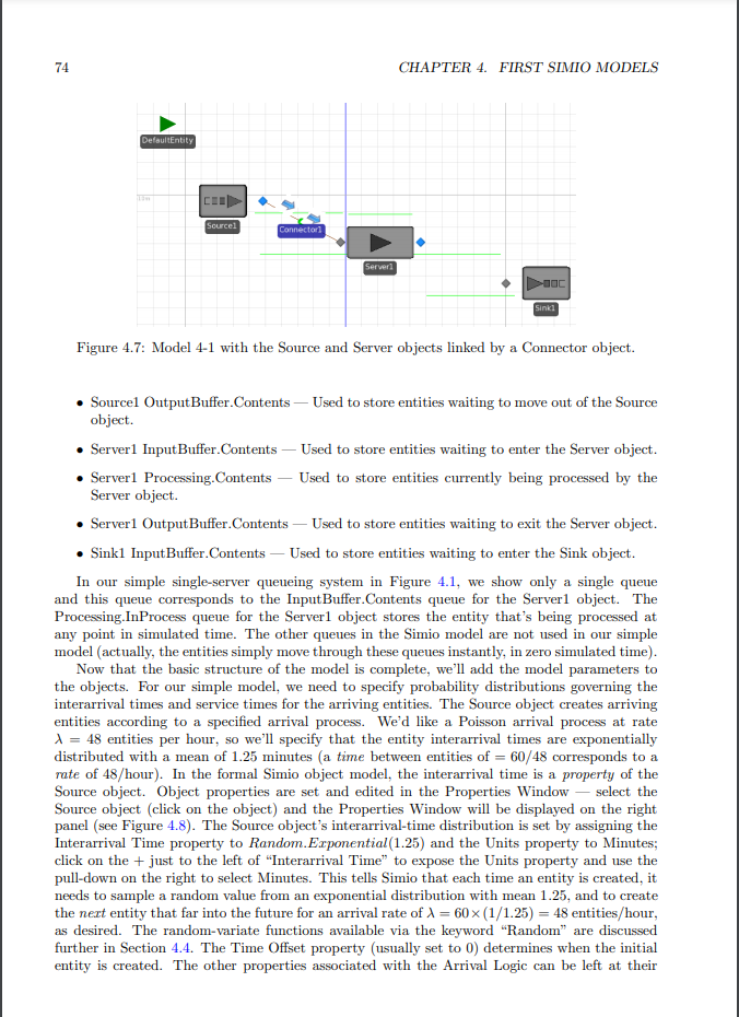
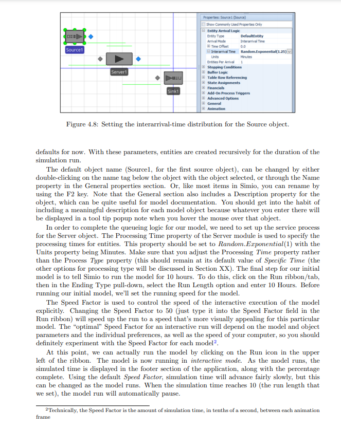
4.11 Problems 1. Create a model similar to Model 4-1 except use an arrival rate, 1, of 120 entities per hour and a service rate, p, of 190 entities per hour. Run your model for 100 hours and report the number of entities that were created, the number that completed service, and the average time entities spend in the system. 2. Develop a queueing model for the Simio model from Problem 1 and compute the exact values for the steady state time entities spend in the system and the expected number of entities processed in 100 hours. 4. If you run the experiment from Problem 3 five (or any number of times, you will always get the exact same results even though the interarrival and service times are supposed to be random. Why is this? 5. You develop a model of a system. As part of your verification, you also develop some expectation about the results that you should get. When you run the model, however, the results do not match your expectations. What are the three possible explanations for this mismatch? 6. In the context of simulation modeling, what is a replication and how, in general, do you determine how many replications to run for a given model? 7. What is the difference between a steady-state simulation and a terminating simulation? 8. What are the initial transient period and the warm-up period for a steady-state simulation? 74 CHAPTER 4. FIRST SIMIO MODELS DefaultEntity Sourcel Connector Server Sinki Figure 4.7: Model 4-1 with the Source and Server objects linked by a Connector object. Sourcel OutputBuffer.Contents Used to store entities waiting to move out of the Source object. Server1 InputBuffer.Contents Used to store entities waiting to enter the Server object. Server1 Processing. Contents Used to store entities currently being processed by the Server object. Server1 OutputBuffer.Contents Used to store entities waiting to exit the Server object. Sinki InputBuffer.Contents - Used to store entities waiting to enter the Sink object. In our simple single-server queueing system in Figure 4.1, we show only a single queue and this queue corresponds to the InputBuffer.Contents queue for the Serverl object. The Processing. In Process queue for the Serverl object stores the entity that's being processed at any point in simulated time. The other queues in the Simio model are not used in our simple model actually, the entities simply move through these queues instantly, in zero simulated time). Now that the basic structure of the model is complete, we'll add the model parameters to the objects. For our simple model, we need to specify probability distributions governing the interarrival times and service times for the arriving entities. The Source object creates arriving entities according to a specified arrival process. We'd like a Poisson arrival process at rate * = 48 entities per hour, so we'll specify that the entity interarrival times are exponentially distributed with a mean of 1.25 minutes a time between entities of = 60/48 corresponds to a rate of 48/hour). In the formal Simio object model, the interarrival time is a property of the Source object. Object properties are set and edited in the Properties Window select the Source object click on the object) and the Properties Window will be displayed on the right panel (see Figure 4.8). The Source object's interarrival-time distribution is set by assigning the Interarrival Time property to Random.Exponential(1.25) and the Units property to Minutes; click on the + just to the left of "Interarrival Time" to expose the Units property and use the pull-down on the right to select Minutes. This tells Simio that each time an entity is created, it needs to sample a random value from an exponential distribution with mean 1.25, and to create the next entity that far into the future for an arrival rate of = 60x (1/1.25) = 48 entities/hour, as desired. The random-variate functions available via the keyword "Random are discussed further in Section 4.4. The Time Offset property (usually set to 0) determines when the initial entity is created. The other properties associated with the Arrival Logic can be left at their Source1 Properties: Source 1 (Source) Show commonly used Properties Only Entity Arrival Log Entity Type Default Entity Arrival Mode Interarnival Time Time Offset 0.0 Interarrival Time Random.Exponential(1.25) Units Minutes Entities Per Arrival 1 Stopping Conditions Buffer Log Table Row Referencing State Assignments ancials Add-On Process Triggers Advanced Options General Animation Server Sink1 Figure 4.8: Setting the interarrival-time distribution for the Source object. defaults for now. With these parameters, entities are created recursively for the duration of the simulation run. The default object name (Sourcel, for the first source object), can be changed by either double-clicking on the name tag below the object with the object selected, or through the Name property in the General properties section. Or, like most items in Simio, you can rename by using the F2 key. Note that the General section also includes a Description property for the object, which can be quite useful for model documentation. You should get into the habit of including a meaningful description for each model object because whatever you enter there will be displayed in a tool tip popup note when you hover the mouse over that object. In order to complete the queueing logic for our model, we need to set up the service process for the Server object. The Processing Time property of the Server module is used to specify the processing times for entities. This property should be set to Random.Erponential(1) with the Units property being Minutes. Make sure that you adjust the Processing Time property rather than the Process Type property (this should remain at its default value of Specific Time (the other options for processing type will be discussed in Section XX). The final step for our initial model is to tell Simio to run the model for 10 hours. To do this, click on the Run ribbon/tab, then in the Ending Type pull-down, select the Run Length option and enter 10 Hours. Before running our initial model, we'll set the running speed for the model. The Speed Factor is used to control the speed of the interactive execution of the model explicitly. Changing the Speed Factor to 50 (just type it into the Speed Factor field in the Run ribbon) will speed up the run to a speed that's more visually appealing for this particular model. The "optimal" Speed Factor for an interactive run will depend on the model and object parameters and the individual preferences, as well as the speed of your computer, so you should definitely experiment with the Speed Factor for each model. At this point, we can actually run the model by clicking on the Run icon in the upper left of the ribbon. The model is now running in interactive mode. As the model runs, the simulated time is displayed in the footer section of the application, along with the percentage complete. Using the default Speed Factor, simulation time will advance fairly slowly, but this can be changed as the model runs. When the simulation time reaches 10 (the run length that we set), the model run will automatically pause. 2 Technically, the Speed Factor is the amount of simulation time, in tenths of a second, between each animation frame