Question: Assignment 4 + 5 : Predicting 1 0 - Day Velocity Components ( u ) and ( v ) Using EOF
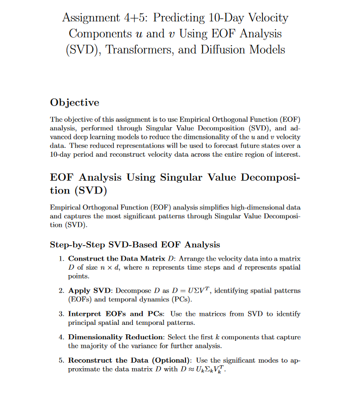
Assignment : Predicting Day Velocity Components u and v Using EOF Analysis SVD Transformers, and Diffusion Models
Objective
The objective of this assignment is to use Empirical Orthogonal Function EOF analysis, performed through Singular Value Decomposition SVD and advanced deep learning models to reduce the dimensionality of the u and v velocity data. These reduced representations will be used to forecast future states over a day period and reconstruct velocity data across the entire region of interest.
EOF Analysis Using Singular Value Decomposition SVD
Empirical Orthogonal Function EOF analysis simplifies highdimensional data and captures the most significant patterns through Singular Value Decomposition SVD
StepbyStep SVDBased EOF Analysis
Construct the Data Matrix D : Arrange the velocity data into a matrix D of size n times d where n represents time steps and d represents spatial points.
Apply SVD: Decompose D as DU Sigma VT identifying spatial patterns EOFs and temporal dynamics PCs
Interpret EOFs and PCs: Use the matrices from SVD to identify principal spatial and temporal patterns.
Dimensionality Reduction: Select the first k components that capture the majority of the variance for further analysis.
Reconstruct the Data Optional: Use the significant modes to approximate the data matrix D with D approx UkSigmak VkT Forecasting with Transformers
Using EOF Analysis
Model Setup: Utilize a transformer model to forecast future velocity components using the Principal Components PCs as input, which are derived from the EOF analysis.
Data Preparation: Format the reduced data from EOF analysis for sequential processing in the transformer. Ensure that the input sequence to the transformer appropriately encapsulates temporal dynamics as represented by the PCs
Implementation Details: 'Train the transformer to predict the future state of the PCs over a day period. The training should focus on capturing the temporal dependencies and dynamics encapsulated by the EOFderived PCs
Without Using EOF Analysis
Model Setup: In this approach, use the transformer to directly forecast future velocity components based on the original, nonreduced data.
Data Preparation: Prepare the original velocity data by structuring it into an appropriate sequence format for the transformer, maintaining the full complexity of the spatialtemporal patterns.
Implementation Details: Train the transformer model on the full dataset to predict the future velocity components over the same day period. This approach tests the transformer's ability to handle highdimensional data without the preprocessing step of dimensionality reduction.
Comparison Task: After completing both forecasting approaches, students are required to compare the performance, efficiency, and accuracy of the forecasts generated by the transformers with and without the use of EOF analysis. Discuss the advantages and potential limitations of each approach.
Reconstruction Using Diffusion Models
Objective: Use a diffusion model to reconstruct the velocities from partial observations of the map to the entire region of interest.
Data Provision: Different data sets will be provided specifically for this task.
Methodology: Implement the diffusion process to generate complete velocity fields from sparse or incomplete data. Task Implementation
EOFs and PCs Extraction: Identify EOFs and PCs through SVD on the data matrix to be used in subsequent forecasting tasks.
Machine Learning Forecasting:
Using EOFderived PCs:
Train LSTM RNN and MLP models on the PCs to predict future values, focusing on capturing the essential dynamics.
Train a Transformer model to forecast the future state of the PCs over a day period, using the reduced representation from EOF analysis.
Using original, nonreduced data:
Train a Transformer model directly on the original, nonreduced data to forecast future velocity components, testing the ability to process complex highdimensional data.
Comparison of Forecasting Methods: Students are required to compare the performance of LSTM RNN MLP and Transformer models when using EOFderived PCs versus using the original dataset in the Transformer model. For this comparison, students should use the following metrics:
Correlation Coefficient: Measure the linear correlation between the actual and forecasted values to evaluate the accuracy and predictive performance of each model.
Mean Squared Error MSE: Calculate the MSE to assess the average squared difference between the estimated values and what is estimated. This metric will help evaluate the precision of the forecast.
Computational Efficiency: Analyze the time and resources required for training and predicting with each model, assessing how well each method handles the complexity and size of the data.
Discuss the advantages and potential limita Evaluate Reconstruction Quality: Assess the quali

Step by Step Solution
There are 3 Steps involved in it
1 Expert Approved Answer
Step: 1 Unlock


Question Has Been Solved by an Expert!
Get step-by-step solutions from verified subject matter experts
Step: 2 Unlock
Step: 3 Unlock


