Assignment

The Assignment B for this Workshop is to perform an analysis which computes the theoretical allocation, the actual allocation, and compares the two. You will be working with daily return data for the Market Index, consisting of 30 stocks. The work involved is the following:

1. Load the necessary data. The required data files are all listed in the Syllabus table under Workshop at the bottom the AMS 511 course page.

1. 1.1. Import[]thedailyreturnvectorforthereturnsoftheMarketIndexwhichwillrepresentthemarket. This is a vector of length 1471 with each element representing a different date.

2. 1.2. Import[]thedailyreturnsmatrixforthethirtymembersoftheMarketIndex.Thisisamatrixof dimension 147130 with each row representing a different date and each column a different stock.

3. 1.3. Bothoftheabovearealignedproperly.

2. Perform a CAPM linear regression to estimate the betas and error variances of each member of the Market Index. For simplicity assume an annual risk free rate of 1.6%. Approximate the daily rate as (1 + 0.016)^(1/250) - 1.

3. Use these estimates of the betas and error variances to compute the proportional allocations of each stock as predicted by the CAPM and normalize them so they sum to one..

4. Import[ ] the actual market capitalization of each of the 30 stocks. Use these data to produce the proportional market allocations.

5. Plot histograms of the empirical PDFs of the betas and error variances. For each case, use the code

   Histogram[data, Automatic, "PDF"]

6. UseListPlot[]toplottheCAPMallocationsestimatedin(3.)vstheobservedbasedon capitalization in (4.).

7. Perform whatever additional comparisons you feel would be useful to characterize what you found.

8. What discrepancies do you note? How might you explain them? Mathematica

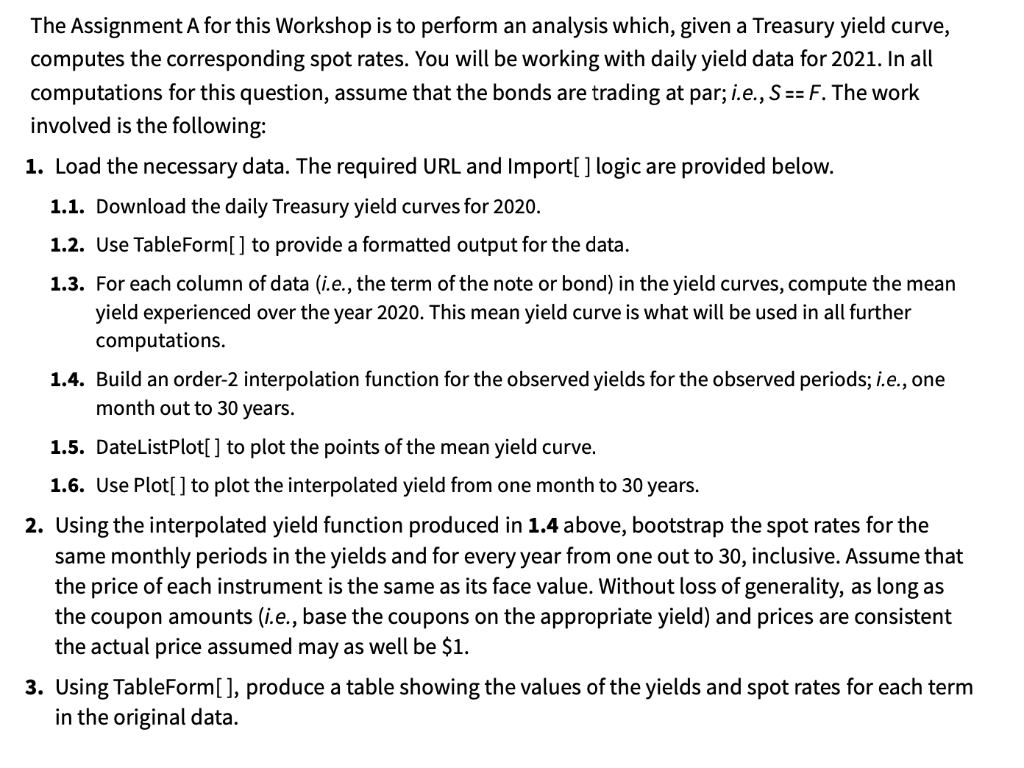
The Assignment A for this Workshop is to perform an analysis which, given a Treasury yield curve, computes the corresponding spot rates. You will be working with daily yield data for 2021. In all computations for this question, assume that the bonds are trading at par; i.e., S == F. The work involved is the following: 1. Load the necessary data. The required URL and Import[] logic are provided below. 1.1. Download the daily Treasury yield curves for 2020. 1.2. Use TableForm[] to provide a formatted output for the data. 1.3. For each column of data (i.e., the term of the note or bond) in the yield curves, compute the mean yield experienced over the year 2020. This mean yield curve is what will be used in all further computations. 1.4. Build an order-2 interpolation function for the observed yields for the observed periods; i.e., one month out to 30 years. 1.5. DateListPlot[] to plot the points of the mean yield curve. 1.6. Use Plot[] to plot the interpolated yield from one month to 30 years. 2. Using the interpolated yield function produced in 1.4 above, bootstrap the spot rates for the same monthly periods in the yields and for every year from one out to 30, inclusive. Assume that the price of each instrument is the same as its face value. Without loss of generality, as long as the coupon amounts (i.e., base the coupons on the appropriate yield) and prices are consistent the actual price assumed may as well be $1. 3. Using TableForm[], produce a table showing the values of the yields and spot rates for each term in the original data. The Assignment A for this Workshop is to perform an analysis which, given a Treasury yield curve, computes the corresponding spot rates. You will be working with daily yield data for 2021. In all computations for this question, assume that the bonds are trading at par; i.e., S == F. The work involved is the following: 1. Load the necessary data. The required URL and Import[] logic are provided below. 1.1. Download the daily Treasury yield curves for 2020. 1.2. Use TableForm[] to provide a formatted output for the data. 1.3. For each column of data (i.e., the term of the note or bond) in the yield curves, compute the mean yield experienced over the year 2020. This mean yield curve is what will be used in all further computations. 1.4. Build an order-2 interpolation function for the observed yields for the observed periods; i.e., one month out to 30 years. 1.5. DateListPlot[] to plot the points of the mean yield curve. 1.6. Use Plot[] to plot the interpolated yield from one month to 30 years. 2. Using the interpolated yield function produced in 1.4 above, bootstrap the spot rates for the same monthly periods in the yields and for every year from one out to 30, inclusive. Assume that the price of each instrument is the same as its face value. Without loss of generality, as long as the coupon amounts (i.e., base the coupons on the appropriate yield) and prices are consistent the actual price assumed may as well be $1. 3. Using TableForm[], produce a table showing the values of the yields and spot rates for each term in the original data