assignment2.py File image

data CSV file

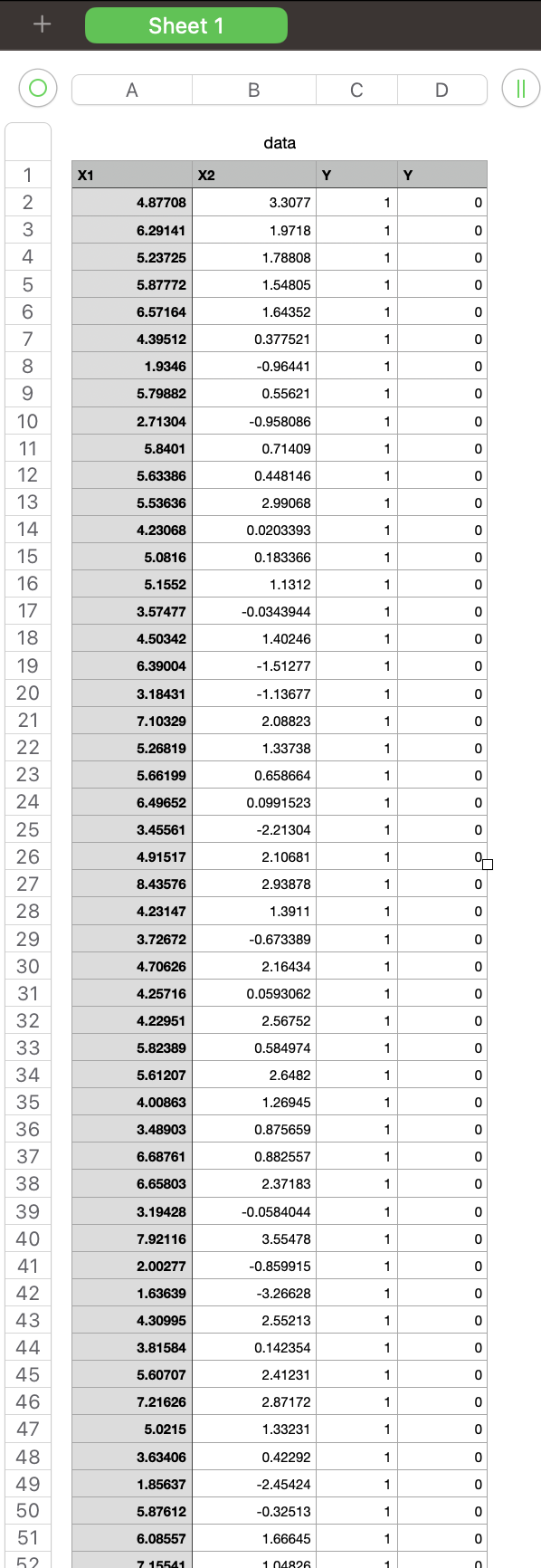
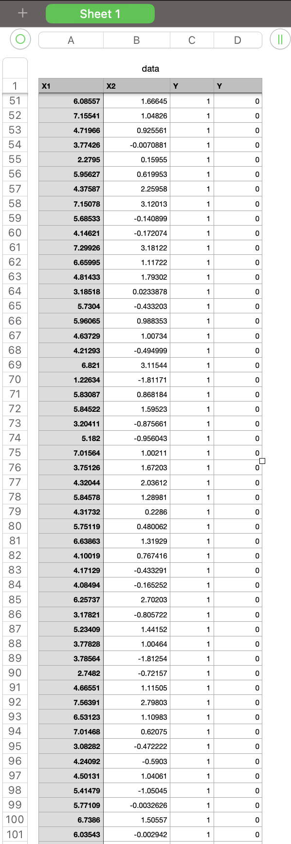
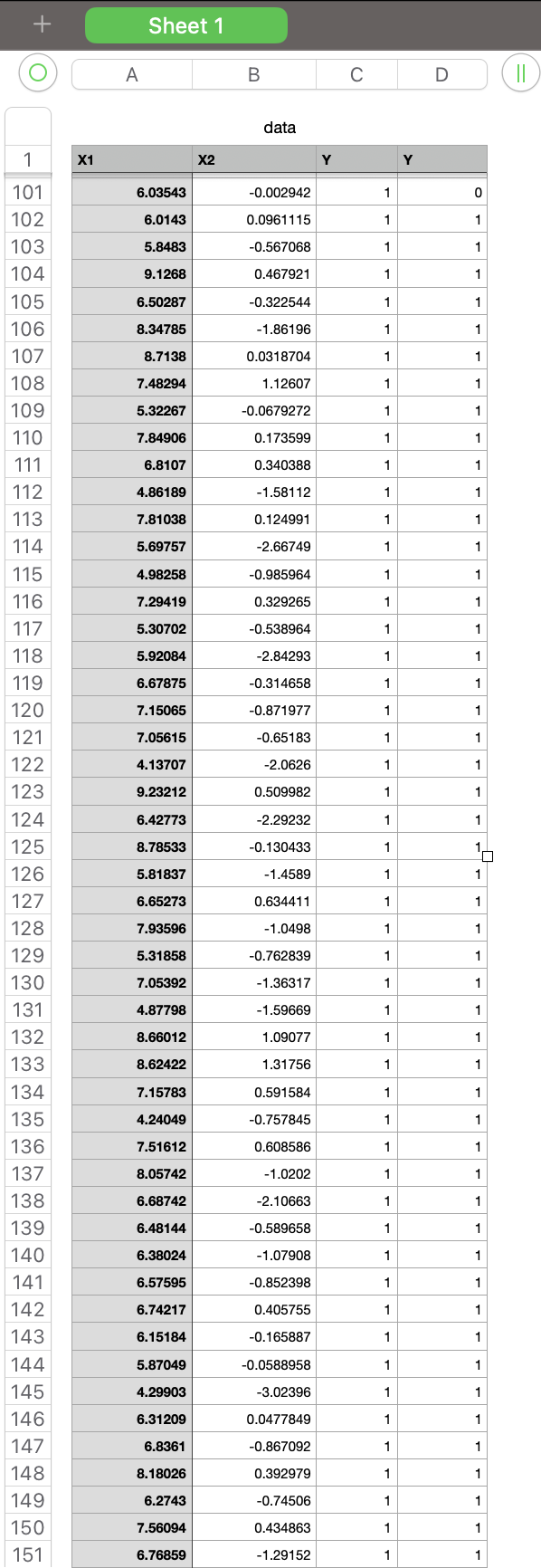
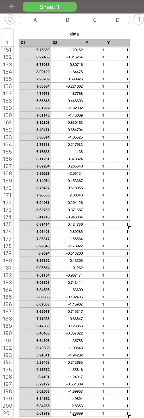
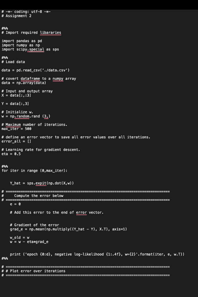
Question 2. (60\%) This question will examine optimization techniques for classification with logistic regression. Download the code file consisting of the assignment2 code and data CSV file. In the data file, the first, second, and third columns are called the inputs dataset and contain the input features. The fourth column is called the outputs dataset and contains the class number for each input sample. Open the script assignment2.py in the Ir directory. This code performs gradient descent to optimize parameters (w) which minimizes the error. The parameters are initialized in the beginning. In the code, the data is loaded, and inputs and output arrays are extracted. Afterward, for 500 iterations, the predicted outputs are computed using the following formula for each iteration. Z=WTXY^=Sigmoid(Z) Now, in order to optimize the parameters and train the model, complete the missing parts in the code under the comment blocks. 1- Compute the error: In the code, the error value is initialized to zero (e=0). Compute the error values using the Logistic Regression Cost Function as follows and replace it with e: Error=m1i=1m[Yilog(Y^i)+(1Yi)log(1Y^i)] Then append the computed error value to the error_all vector in order to save your error in all iterations. 2- Plot the error values during the iterations and explain why this plot is oscillating. 3- Create a Python script named assignment2_q2_3.py for the following. Modify assignment2.py to run gradient descent with the learning rates = 0:5,0:3,0:1,0:05,0:01. Include in your report a single plot comparing error values versus iterations for these different learning rates. Compare these results. What are the relative advantages of the different rates? 4- Create a Python script named assignment2_q2_4.py for the following. Modify this code to do stochastic gradient descent. Use the parameters = 0:5,0:3,0:1,0:05,0:01. 2 Include in your report a new plot comparing error values versus iterations using stochastic gradient descent. Is stochastic gradient descent faster than gradient descent? Explain using your plots. Submission: Submit two files: 1. A PDF file containing the solutions to question 1 and the figures/explanations requested for question 2. Save your file as FirstName-LastName.PDF. 2. A zip file of all your code, called code.zip. \# -*- coding: utf-8 -*- \# Assignment 2 \# Import required libararies import pandas as pd import numpy as np import scipy.special as sps \# Load data data = pd.read_csv('./data. csv) \# covert dataframe to a numpy array data =np,array( data) \# Input and output array X=data[:,:3] Y=data[:,3] \# Initialize w. w=np random. rand (3, \# Maximum number of iterations. max_iter =500 \# define an error vector to save all error values over all iterations. error_all = [] \# Learning rate for gradient descent. eta =0.5 for iter in range (0, max iter ): Y_hat =sps,expit(np,dot(X,w)) \# Gradient of the error grad_e =np.mean(np.multiply((Y_hat Y),X.T), axis =1) wold=w w=w eta*grad_e print ('epoch {0:d}, negative log-likelihood {1:.4f},w={2} ', format(iter, e, w.T) ) \# \# Plot error over iterations + Sheet 1 \begin{tabular}{|l|l|l|l|} \hlineA & B & C & D \\ \hline \end{tabular} data \begin{tabular}{|c|} \hline 1 \\ \hline 2 \\ \hline 3 \\ \hline 4 \\ \hline 5 \\ \hline 6 \\ \hline 7 \\ \hline 8 \\ \hline 9 \\ \hline 10 \\ \hline 11 \\ \hline 12 \\ \hline 13 \\ \hline 14 \\ \hline 51 \\ \hline 15 \\ \hline 16 \\ \hline 48 \\ \hline 17 \\ \hline 46 \\ \hline 18 \\ \hline 19 \\ \hline 43 \\ \hline 40 \\ \hline 43 \\ \hline 21 \\ \hline \hline \\ \hline 22 \\ \hline 23 \\ \hline 24 \\ \hline 25 \\ \hline 26 \\ \hline 27 \\ \hline 28 \\ \hline 29 \\ \hline 30 \\ \hline 31 \\ \hline 32 \\ \hline 33 \\ \hline 34 \\ \hline 35 \\ \hline 36 \\ \hline \end{tabular} Sheet 1 \begin{tabular}{|l|l|l|l|} \hline A & B & C & D \\ \hline \end{tabular} (11) data \begin{tabular}{|c|r|r|r|r|} \hline \multicolumn{1}{|c|}{} & \multicolumn{1}{|l|}{ Sheet 1} & & & \\ \hline & & & \\ \hline & & & & \\ \hline \end{tabular} Sheet 1 \begin{tabular}{|l|l|l|l|} \hline A & B & C & D \\ \hline \end{tabular} (II) data