Assume that we observe two different processes in real-life and collect data associated with these processes....

 

Transcribed Image Text:

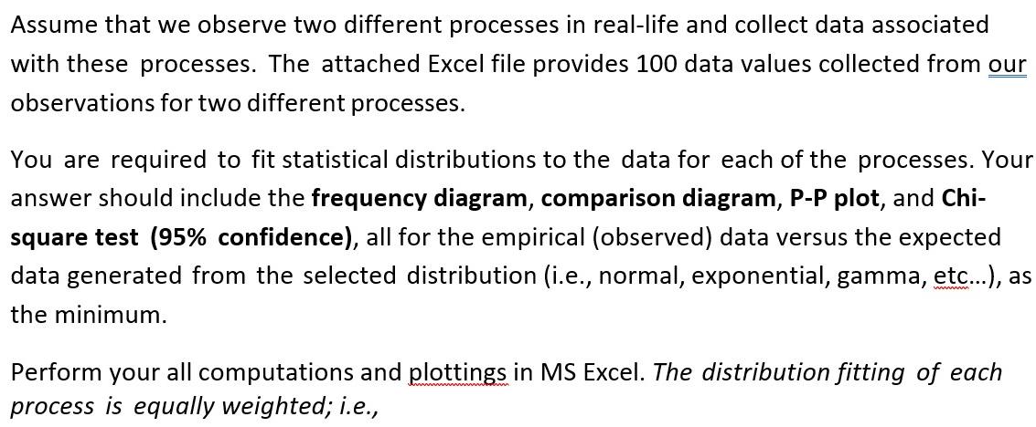
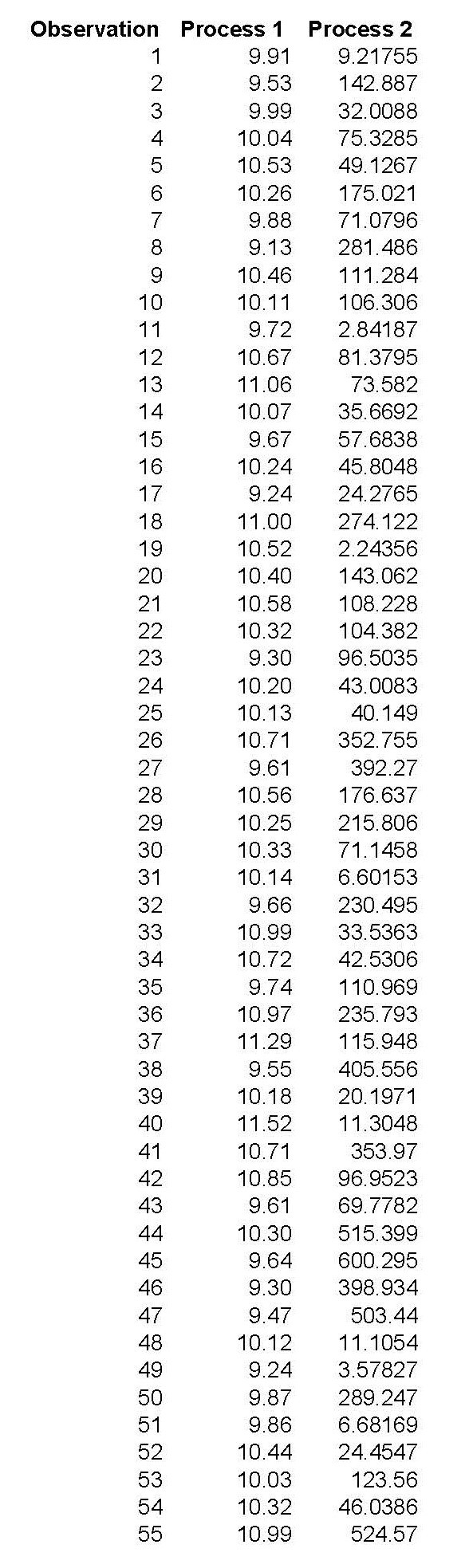
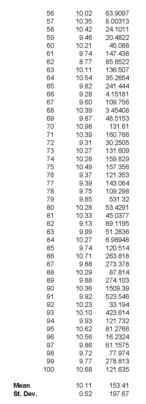
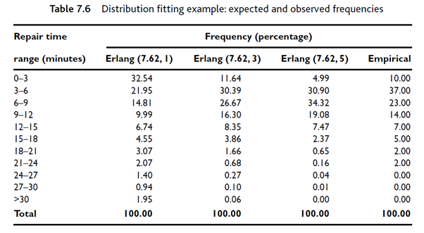
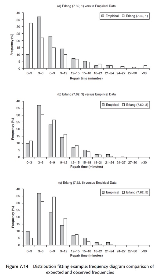
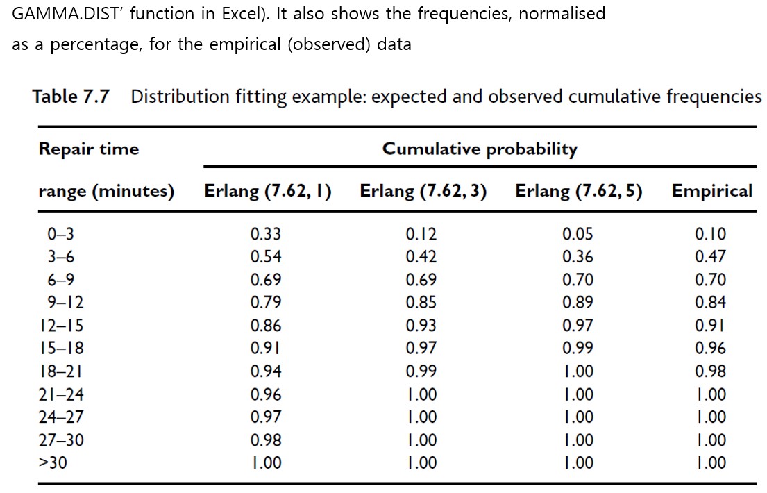
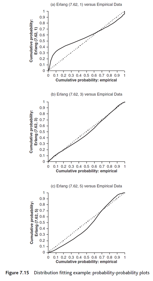
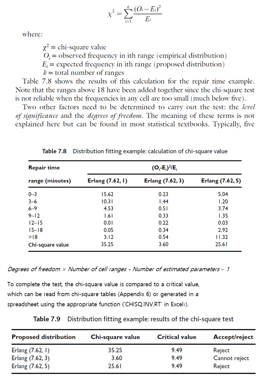
Assume that we observe two different processes in real-life and collect data associated with these processes. The attached Excel file provides 100 data values collected from our observations for two different processes. You are required to fit statistical distributions to the data for each of the processes. Your answer should include the frequency diagram, comparison diagram, P-P plot, and Chi- square test (95% confidence), all for the empirical (observed) data versus the expected data generated from the selected distribution (i.e., normal, exponential, gamma, etc...), as the minimum. Perform your all computations and plottings in MS Excel. The distribution fitting of each process is equally weighted; i.e., Observation Process 1 Process 2 12345678 9.91 9.21755 9.53 142.887 9.99 32.0088 10.04 75.3285 10.53 49.1267 10.26 175.021 9.88 71.0796 9.13 281.486 9 10.46 111.284 10 10.11 106.306 11 9.72 2.84187 12 10.67 81.3795 13 11.06 73.582 14 10.07 35.6692 15 9.67 57.6838 16 10.24 45.8048 17 9.24 24.2765 18 11.00 274.122 19 10.52 2.24356 20 10.40 143.062 21 10,58 108.228 22 10.32 104.382 23 9.30 96.5035 24 10.20 43.0083 25 10.13 40.149 26 10.71 352.755 27 9.61 392.27 28 10.56 176.637 29 10.25 215.806 30 10.33 71.1458 31 10.14 6.60153 32 9.66 230.495 33 10.99 33.5363 34 10.72 42.5306 35 9.74 110.969 36 10.97 235.793 37 11.29 115.948 38 9.55 405,556 39 10.18 20.1971 40 11.52 11.3048 41 10.71 353.97 42 10.85 96.9523 43 9.61 69.7782 44 10.30 515.399 45 9.64 600.295 46 9.30 398.934 47 9.47 503.44 48 10.12 11.1054 49 9.24 3.57827 50 9.87 289.247 51 9.86 6.68169 52 10.44 24.4547 53 10.03 123.56 54 10.32 46.0386 55 10.99 524.57 Mean St. Dev. 56 10.02 63.9097 57 10.35 8.00313 58 10.42 24.1011 59 9.46 20.4822 60 10.21 45.088 61 9.74 147.438 62 8.77 85.8522 63 10.11 136.507 64 10.54 35.2654 65 9.82 241.444 66 9.28 4.15181 67 9.60 109.756 68 10.39 3.45408 69 9.87 48.5153 70 10.98 131.61 71 10.39 160,766 72 9.31 30.2505 73 10.27 131.609 74 10.28 159.829 75 10.49 157.356 76 9.37 121.353 77 9.39 143.064 78 9.75 109.298 79 9.85 531.32 80 10.28 53.4291 81 10.33 45.0377 82 9.13 89.1195 83 9.99 51.2836 84 10.27 6.98948 85 9.74 120.514 86 10.71 263.818 87 9.88 273.378 88 10.29 87.814 89 9.88 274.103 90 10.36 1509.39 91 9.92 523.546 92 10.23 33.194 93 10.10 423.614 94 9.93 121.732 95 10.62 81.2766 96 10.56 16.2324 97 9.86 61.1575 98 9.72 77.974 99 9.77 278.813 100 10.68 121.635 10.11 153.41 0.52 197.67 Table 7.6 Distribution fitting example: expected and observed frequencies Repair time Frequency (percentage) range (minutes) Erlang (7.62, 1) Erlang (7.62,3) Erlang (7.62,5) Empirical 0-3 32.54 11.64 4.99 10.00 3-6 6-9 21.95 30.39 30.90 37.00 14.81 26.67 34.32 23.00 9-12 9.99 16.30 19.08 14.00 12-15 6.74 8.35 7.47 7.00 15-18 4.55 3.86 2.37 5.00 18-21 3.07 1.66 0.65 2.00 21-24 2.07 0.68 0.16 2.00 24-27 1.40 0.27 0.04 0.00 27-30 0.94 0.10 0.01 0.00 >30 1.95 0.06 0.00 0.00 Total 100.00 100.00 100.00 100.00 40 35 30 25 20 2250 10 Frequency (%) 50 (a) Erlang (7.62, 1) versus Empirical Data Empirical Erlang (7.62, 1) 0+ 0-3 3-6 6-9 9-12 12-15 15-18 18-21 21-24 24-27 27-30 >30 Repair time (minutes) Empirical Erlang (7.62, 3) 40 (b) Erlang (7.62, 3) versus Empirical Data 35 30- 25 20 15 2 3 3 2 2 50 10 Frequency (%) 50 0-3 Frequency (%) 20 15 NNW & 30 25 40 35 3-6 6-9 9-12 12-15 15-18 18-21 21-24 24-27 27-30 Repair time (minutes) >30 10 5 0-3 3-6 (c) Erlang (7.62, 5) versus Empirical Data Empirical Erlang (7.62, 5) 6-9 9-12 12-15 15-18 18-21 21-24 24-27 27-30 >30 Repair time (minutes) Figure 7.14 Distribution fitting example: frequency diagram comparison of expected and observed frequencies GAMMA.DIST' function in Excel). It also shows the frequencies, normalised as a percentage, for the empirical (observed) data Table 7.7 Distribution fitting example: expected and observed cumulative frequencies Repair time Cumulative probability range (minutes) Erlang (7.62, 1) Erlang (7.62, 3) Erlang (7.62, 5) Empirical 0-3 0.33 0.12 0.05 0.10 3-6 0.54 0.42 0.36 0.47 6-9 0.69 0.69 0.70 0.70 9-12 0.79 0.85 0.89 0.84 12-15 0.86 0.93 0.97 0.91 15-18 0.91 0.97 0.99 0.96 18-21 0.94 0.99 1.00 0.98 21-24 0.96 1.00 1.00 1.00 24-27 0.97 1.00 1.00 1.00 27-30 0.98 1.00 1.00 1.00 >30 1.00 1.00 1.00 1.00 Cumulative probability: Erlang (7.62, 1) Cumulative probability: Erlang (7.62, 3) Cumulative probability: Erlang (7.62, 5) 1 0.9 0.8 65 0.6 0.5 0.4 0.3 0.2 0.1 0 0.9 0.8 7654 3 2 0.5 0.4 0.3 (a) Erlang (7.62, 1) versus Empirical Data 0 0.1 0.2 0.3 0.4 0.5 0.6 0.7 0.8 0.9 1 Cumulative probability: empirical (b) Erlang (7.62, 3) versus Empirical Data 0.2- 0.1 0 0 0.1 0.2 0.3 0.4 0.5 0.6 0.7 0.8 0.9 1 Cumulative probability: empirical 0.9 0.8 0.6 0.5 0.4 0.3 0.2 (c) Erlang (7.62, 5) versus Empirical Data 0.1 0 0 0.1 0.2 0.3 0.4 0.5 0.6 0.7 0.8 0.9 1 Cumulative probability: empirical Figure 7.15 Distribution fitting example: probability-probability plots Ei i=1 where: x2 chi-square value = O; observed frequency in ith range (empirical distribution) E;= expected frequency in ith range (proposed distribution) k = total number of ranges Table 7.8 shows the results of this calculation for the repair time example. Note that the ranges above 18 have been added together since the chi-square test is not reliable when the frequencies in any cell are too small (much below five). Two other factors need to be determined to carry out the test: the level of significance and the degrees of freedom. The meaning of these terms is not explained here but can be found in most statistical textbooks. Typically, five Table 7.8 Distribution fitting example: calculation of chi-square value Repair time range (minutes) (O-E)/E Erlang (7.62, 1) Erlang (7.62, 3) Erlang (7.62,5) 0-3 15.62 0.23 5.04 3-6 10.31 1.44 1.20 6-9 4.53 0.51 3.74 9-12 1.61 0.33 1.35 12-15 0.01 0.22 0.03 15-18 0.05 0.34 2.92 >18 3.12 0.54 11.32 Chi-square value 35.25 3.60 25.61 Degrees of freedom = Number of cell ranges - Number of estimated parameters - 1 To complete the test, the chi-square value is compared to a critical value, which can be read from chi-square tables (Appendix 6) or generated in a spreadsheet using the appropriate function ('CHISQ. INV.RT' in Excel1). Table 7.9 Distribution fitting example: results of the chi-square test Proposed distribution Chi-square value Critical value Accept/reject Erlang (7.62, 1) 35.25 9.49 Reject Erlang (7.62, 3) 3.60 9.49 Cannot reject Erlang (7.62, 5) 25.61 9.49 Reject Assume that we observe two different processes in real-life and collect data associated with these processes. The attached Excel file provides 100 data values collected from our observations for two different processes. You are required to fit statistical distributions to the data for each of the processes. Your answer should include the frequency diagram, comparison diagram, P-P plot, and Chi- square test (95% confidence), all for the empirical (observed) data versus the expected data generated from the selected distribution (i.e., normal, exponential, gamma, etc...), as the minimum. Perform your all computations and plottings in MS Excel. The distribution fitting of each process is equally weighted; i.e., Observation Process 1 Process 2 12345678 9.91 9.21755 9.53 142.887 9.99 32.0088 10.04 75.3285 10.53 49.1267 10.26 175.021 9.88 71.0796 9.13 281.486 9 10.46 111.284 10 10.11 106.306 11 9.72 2.84187 12 10.67 81.3795 13 11.06 73.582 14 10.07 35.6692 15 9.67 57.6838 16 10.24 45.8048 17 9.24 24.2765 18 11.00 274.122 19 10.52 2.24356 20 10.40 143.062 21 10,58 108.228 22 10.32 104.382 23 9.30 96.5035 24 10.20 43.0083 25 10.13 40.149 26 10.71 352.755 27 9.61 392.27 28 10.56 176.637 29 10.25 215.806 30 10.33 71.1458 31 10.14 6.60153 32 9.66 230.495 33 10.99 33.5363 34 10.72 42.5306 35 9.74 110.969 36 10.97 235.793 37 11.29 115.948 38 9.55 405,556 39 10.18 20.1971 40 11.52 11.3048 41 10.71 353.97 42 10.85 96.9523 43 9.61 69.7782 44 10.30 515.399 45 9.64 600.295 46 9.30 398.934 47 9.47 503.44 48 10.12 11.1054 49 9.24 3.57827 50 9.87 289.247 51 9.86 6.68169 52 10.44 24.4547 53 10.03 123.56 54 10.32 46.0386 55 10.99 524.57 Mean St. Dev. 56 10.02 63.9097 57 10.35 8.00313 58 10.42 24.1011 59 9.46 20.4822 60 10.21 45.088 61 9.74 147.438 62 8.77 85.8522 63 10.11 136.507 64 10.54 35.2654 65 9.82 241.444 66 9.28 4.15181 67 9.60 109.756 68 10.39 3.45408 69 9.87 48.5153 70 10.98 131.61 71 10.39 160,766 72 9.31 30.2505 73 10.27 131.609 74 10.28 159.829 75 10.49 157.356 76 9.37 121.353 77 9.39 143.064 78 9.75 109.298 79 9.85 531.32 80 10.28 53.4291 81 10.33 45.0377 82 9.13 89.1195 83 9.99 51.2836 84 10.27 6.98948 85 9.74 120.514 86 10.71 263.818 87 9.88 273.378 88 10.29 87.814 89 9.88 274.103 90 10.36 1509.39 91 9.92 523.546 92 10.23 33.194 93 10.10 423.614 94 9.93 121.732 95 10.62 81.2766 96 10.56 16.2324 97 9.86 61.1575 98 9.72 77.974 99 9.77 278.813 100 10.68 121.635 10.11 153.41 0.52 197.67 Table 7.6 Distribution fitting example: expected and observed frequencies Repair time Frequency (percentage) range (minutes) Erlang (7.62, 1) Erlang (7.62,3) Erlang (7.62,5) Empirical 0-3 32.54 11.64 4.99 10.00 3-6 6-9 21.95 30.39 30.90 37.00 14.81 26.67 34.32 23.00 9-12 9.99 16.30 19.08 14.00 12-15 6.74 8.35 7.47 7.00 15-18 4.55 3.86 2.37 5.00 18-21 3.07 1.66 0.65 2.00 21-24 2.07 0.68 0.16 2.00 24-27 1.40 0.27 0.04 0.00 27-30 0.94 0.10 0.01 0.00 >30 1.95 0.06 0.00 0.00 Total 100.00 100.00 100.00 100.00 40 35 30 25 20 2250 10 Frequency (%) 50 (a) Erlang (7.62, 1) versus Empirical Data Empirical Erlang (7.62, 1) 0+ 0-3 3-6 6-9 9-12 12-15 15-18 18-21 21-24 24-27 27-30 >30 Repair time (minutes) Empirical Erlang (7.62, 3) 40 (b) Erlang (7.62, 3) versus Empirical Data 35 30- 25 20 15 2 3 3 2 2 50 10 Frequency (%) 50 0-3 Frequency (%) 20 15 NNW & 30 25 40 35 3-6 6-9 9-12 12-15 15-18 18-21 21-24 24-27 27-30 Repair time (minutes) >30 10 5 0-3 3-6 (c) Erlang (7.62, 5) versus Empirical Data Empirical Erlang (7.62, 5) 6-9 9-12 12-15 15-18 18-21 21-24 24-27 27-30 >30 Repair time (minutes) Figure 7.14 Distribution fitting example: frequency diagram comparison of expected and observed frequencies GAMMA.DIST' function in Excel). It also shows the frequencies, normalised as a percentage, for the empirical (observed) data Table 7.7 Distribution fitting example: expected and observed cumulative frequencies Repair time Cumulative probability range (minutes) Erlang (7.62, 1) Erlang (7.62, 3) Erlang (7.62, 5) Empirical 0-3 0.33 0.12 0.05 0.10 3-6 0.54 0.42 0.36 0.47 6-9 0.69 0.69 0.70 0.70 9-12 0.79 0.85 0.89 0.84 12-15 0.86 0.93 0.97 0.91 15-18 0.91 0.97 0.99 0.96 18-21 0.94 0.99 1.00 0.98 21-24 0.96 1.00 1.00 1.00 24-27 0.97 1.00 1.00 1.00 27-30 0.98 1.00 1.00 1.00 >30 1.00 1.00 1.00 1.00 Cumulative probability: Erlang (7.62, 1) Cumulative probability: Erlang (7.62, 3) Cumulative probability: Erlang (7.62, 5) 1 0.9 0.8 65 0.6 0.5 0.4 0.3 0.2 0.1 0 0.9 0.8 7654 3 2 0.5 0.4 0.3 (a) Erlang (7.62, 1) versus Empirical Data 0 0.1 0.2 0.3 0.4 0.5 0.6 0.7 0.8 0.9 1 Cumulative probability: empirical (b) Erlang (7.62, 3) versus Empirical Data 0.2- 0.1 0 0 0.1 0.2 0.3 0.4 0.5 0.6 0.7 0.8 0.9 1 Cumulative probability: empirical 0.9 0.8 0.6 0.5 0.4 0.3 0.2 (c) Erlang (7.62, 5) versus Empirical Data 0.1 0 0 0.1 0.2 0.3 0.4 0.5 0.6 0.7 0.8 0.9 1 Cumulative probability: empirical Figure 7.15 Distribution fitting example: probability-probability plots Ei i=1 where: x2 chi-square value = O; observed frequency in ith range (empirical distribution) E;= expected frequency in ith range (proposed distribution) k = total number of ranges Table 7.8 shows the results of this calculation for the repair time example. Note that the ranges above 18 have been added together since the chi-square test is not reliable when the frequencies in any cell are too small (much below five). Two other factors need to be determined to carry out the test: the level of significance and the degrees of freedom. The meaning of these terms is not explained here but can be found in most statistical textbooks. Typically, five Table 7.8 Distribution fitting example: calculation of chi-square value Repair time range (minutes) (O-E)/E Erlang (7.62, 1) Erlang (7.62, 3) Erlang (7.62,5) 0-3 15.62 0.23 5.04 3-6 10.31 1.44 1.20 6-9 4.53 0.51 3.74 9-12 1.61 0.33 1.35 12-15 0.01 0.22 0.03 15-18 0.05 0.34 2.92 >18 3.12 0.54 11.32 Chi-square value 35.25 3.60 25.61 Degrees of freedom = Number of cell ranges - Number of estimated parameters - 1 To complete the test, the chi-square value is compared to a critical value, which can be read from chi-square tables (Appendix 6) or generated in a spreadsheet using the appropriate function ('CHISQ. INV.RT' in Excel1). Table 7.9 Distribution fitting example: results of the chi-square test Proposed distribution Chi-square value Critical value Accept/reject Erlang (7.62, 1) 35.25 9.49 Reject Erlang (7.62, 3) 3.60 9.49 Cannot reject Erlang (7.62, 5) 25.61 9.49 Reject