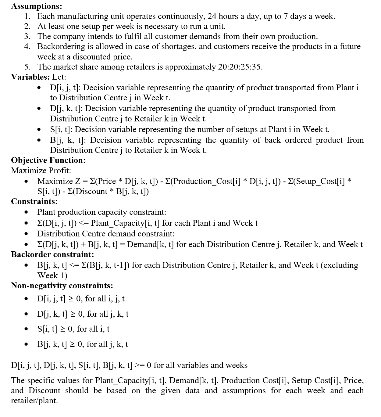
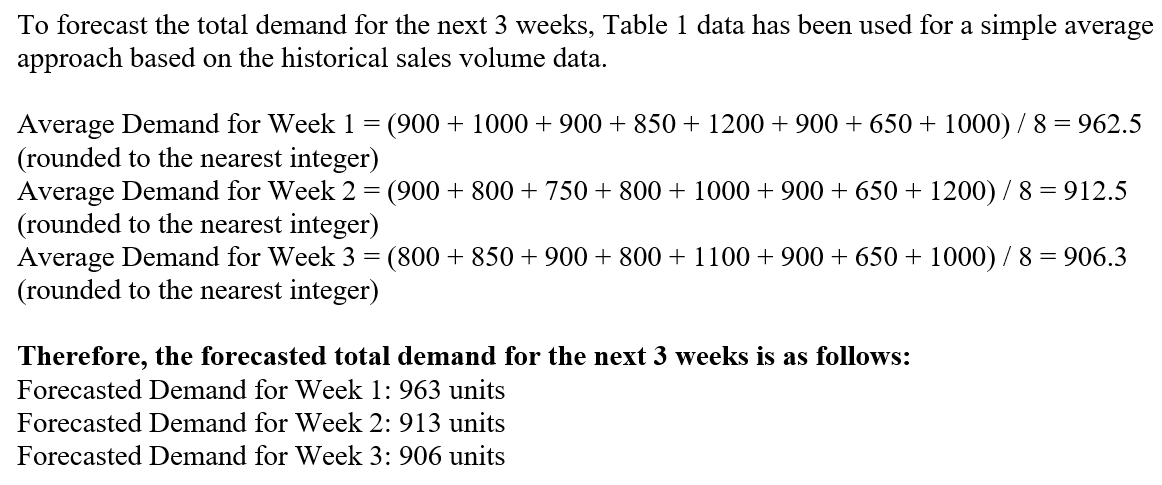
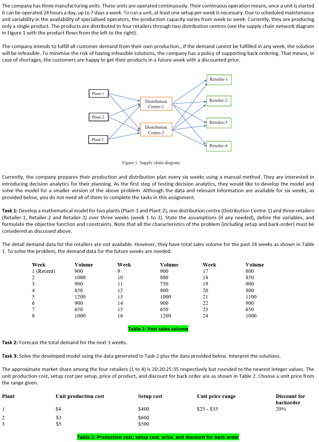
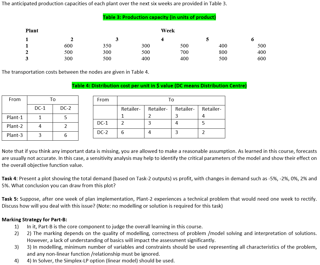
Assumptions: 1. Each manufacturing unit operates continuously, 24 hours a day, up to 7 days a week. 2. At least one setup per week is necessary to run a unit. 3. The company intends to full all customer demands from their own production. 4. Backordering is allowed in case of shortages, and customers receive the products in a future week at a discounted price. 5. The market share among retailers is approximately 2020:2535. Variables: Let: I D[i, j, t]: Decision variable representing the quantity of product transported from Plant i to Distribution Centre j in Week t. 0 D[j, k, t]: Decision variable representing the quantity of product transported from Distribution Centre j to Retailer k in Week t. I S[i, t]: Decision variable representing the number of setups at Plant i in Week t. I B[j_, k, t]: Decision variable representing the quantity of back ordered product from Distribution Centre j to Retailer k in Week t. Objective Function: Maximize Prot: 0 Maximize Z = 2(Price \"5' D[j, k, t]) - E(Production_Cost[i] * D[i,_j, t]) - Z(Setup_Cost[i] \"5' S[i._ t]) - 2(Discount * BU, k, t]) Constraints: 0 Plant production capacity constraint: 0 2-(D[i, j, t]) <: plant_capacity t for each plant i and week distribution centre demand constraint: k b j retailer backorder e t-l weekt non-negativity constraints: d all du s allj bu>= 0 for all variables and weeks The specic values for Plant_Capacity[i, t], Demand[k, t], Production Cost[i], Setup Cost[i], Price, and Discount should be based on the given data and assumptions for each week and each retailer/plant. To forecast the total demand for the next 3 weeks, Table 1 data has been used for a simple average approach based on the historical sales volume data. Average Demand for Week 1 = (900 -- 1000 + 900 + 850 + 1200 + 900 + 650 + 1000) / 8 = 962.5 (rounded to the nearest integer) Average Demand for Week 2 = (900 -- 800 + 750 + 800 + 1000 900 650 1200) / 8 = 912.5 (rounded to the nearest integer) Average Demand for Week 3 = (800 -- 850 + 900 + 800 + 1100 900 650 1000) / 8 = 906.3 (rounded to the nearest integer) Therefore, the forecasted total demand for the next 3 weeks is as follows: Forecasted Demand for Week 1: 963 units Forecasted Demand for Week 2: 913 units Forecasted Demand for Week 3: 906 units The company has three manufacturing units. These units are operated continuously. Their continuous operation means, once a unit is started it can be operated 24 hours a day, up to 7 days a week. To run a unit, at least one setup per week is necessary. Due to scheduled maintenance and variability in the availability of specialised operators, the production capacity varies from week to week. Currently, they are producing only a single product. The products are distributed to four retailers through two distribution centres (see the supply chain network diagram in Figure 1 with the product flows from the left to the right}. The company intends to fulfill all customer demand from their own production, it the demand cannot be fulfilled in any week, the solution will be infeasible. To minimise the risk of having infeasible solutions, the company has a policy of supporting back ordering. That means, in case of shortages, the customers are happy to get their products in a future week with a discounted price. Retailer-l Retailer2 R emiler-R Distribution Centre-2 Retailer-4 Figure l : Supply chain diagram Currently, the company prepares their production and distribution plan every six weeks using a manual method. They are interested in introducing decision analytics for their planning. As the first step of testing decision analytics, they would like to develop the model and solve the model for a smaller version of the above problem. Although the data and relevant information are available for six weeks, as provided below, you do not need all of them to complete the tasks in this assignment. Task 1: Develop a mathematical model fortwo plants (Plant1 and Plant2], one distribution centre (Distribution Centre1) and three retailers (Retailer1, Retailer2 and Retailer3] over three weeks (week 1 to 3). State the assumptions [if any needed}, define the variables, and formulate the objective function and constraints. Note that all the characteristics of the problem [including setup and backorder} must be considered as discussed above. The detail demand data for the retailers are not available. However, they have total sales volume for the past 24 weeks as shown in Table 1. To solve the problem, the demand data for the future weeks are needed. Week Volume Week Volume Week Volume 1 (Recent) 900 9 900 17 800 2 1000 10 800 18 850 3 900 11 750 19 900 4 850 12 800 20 800 5 1200 13 1000 21 1100 6 900 14 900 22 900 7 650 15 650 23 650 8 1000 16 1200 24 1000 Table 1: Past sales volume Task 2: Forecast the total demand for the next 3 weeks. Task 3: Solve the developed model using the data generated in Task2 plus the data provided below. Interpret the solutions. The approximate market share among the four retailers (l to 4] is 2020:2535 respectively but rounded to the nearest integer values. The unit production cost, setup cost per setup, price of product, and discount for back order are as shown in Table 2. Choose a unit price from the range given. Plant Unit production cost Setup cost Unit price range Discount for backorder 1 $4 $400 $25 - $35 20% 2 $3 $600 3 $5 $500 Table 2: Production cost, setup cost, prioe, and discount for back order The anticipated production capacities of each plant over the next six weeks are provided in Table 3. Table 3: Production capacity [in units of product) Plant Week 1 2 3 4 5 6 1 600 350 300 500 400 500 2 500 300 500 7'00 800 400 3 300 500 400 400 500 600 The transportation costs between the nodes are given in Table 4. Table 4: Distribution cost per unit in 5 value [DC means Distribution Centre] From To From To DC-1 DC-2 Retailer Retailer Retailer Retailer Plant1 5 1 2 3 4 Plant2 4 2 D01 2 3 4 5 Plant3 3 6 D02 6 4 3 2 Note that i: you think any important data is missing, you are allowed to make a reasonable assumption. As learned in this course, forecasts are usually not accurate. In this case, a sensitivity analysis may help to identify the critical parameters of the model and show their effect on the overall objective function value. Task4: Present a plot showing the total demand [based on Task2 outputs] vs profit, with changes in demand such as 5%, 2%, 0%, 2% and 5%. What conclusion you can draw from this plot? Task 5: Suppose, after one week of plan implementation, Plant2 experiences a technical problem that would need one week to rectify. Discuss how will you deal with this issue? (Note: no modelling or solution is required for this task) Marking Strategy for Part-B: 1} In it, PartB is the core component to judge the overall learning in this course. 2} 2) The marking depends on the quality of modelling, correctness of problem [model solving and interpretation of solutions. However, a lack of understanding of basics will impact the assessment significantly. 3} 3) In modelling, minimum number of variables and constraints should be used representing all characteristics of the problem, and any nonlinear function [relationship must be ignored. 4} 4) In Solver, the Simplex-LP option {linear model] should be used