AutoParts Analysis.xlsx.

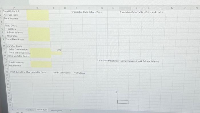
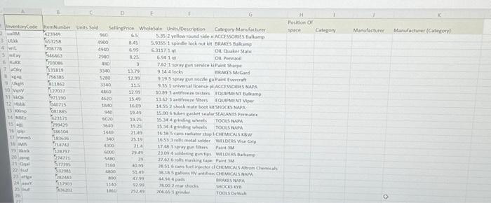
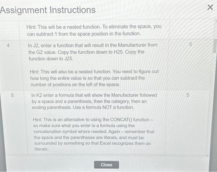
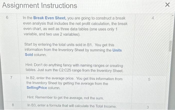
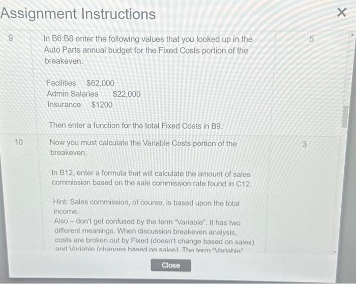
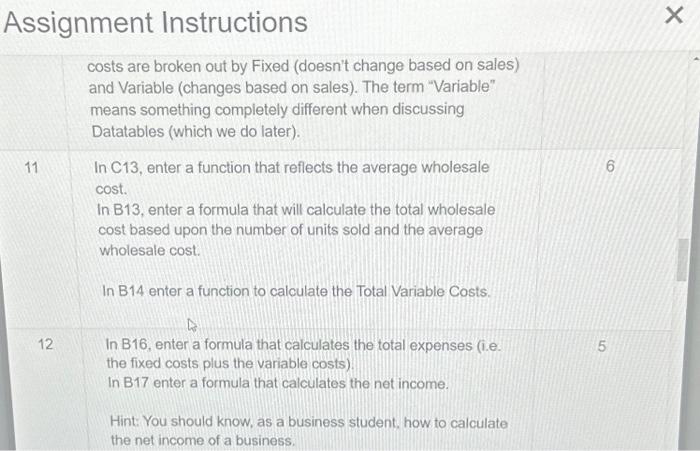
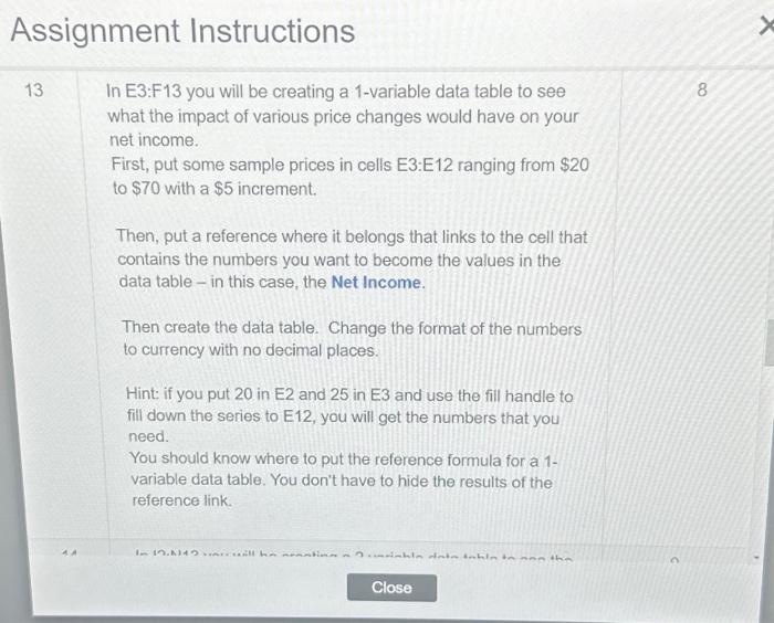
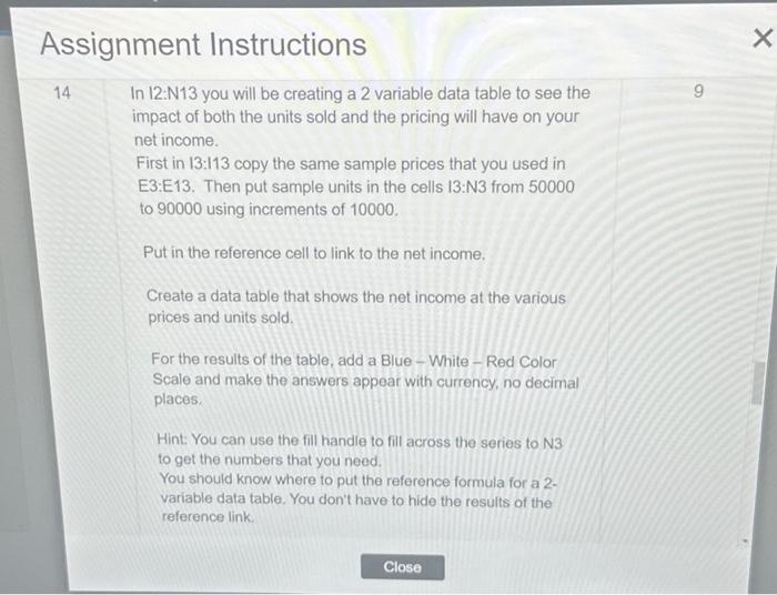
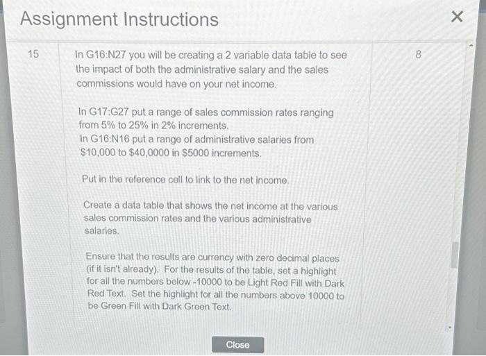
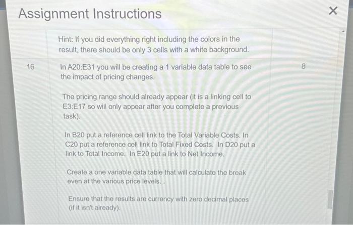
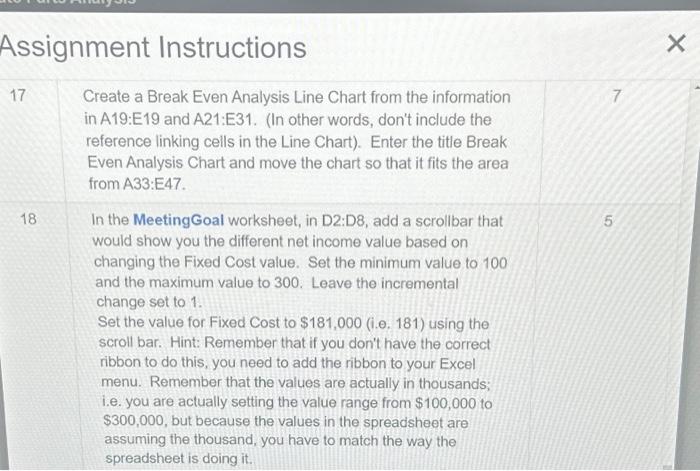
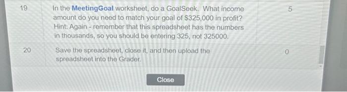
Assignment Instructions As 1,1,1, Assignment Instructions 6 In the Break Even Sheet, you are going to construct a break 4 even analysis that includes the net profit calculation, the break even chart, as well as three data tables (one uses only 1 variable, and two use 2 variables). Start by entering the total units sold in B1. You get this information from the Inventory Sheet by summing the Units Sold column. Hint: Don't do anything fancy with naming ranges or creating tables, Just sum the C2:C25 range from the Inventory Sheet. 7 In B2, enter the average price. You get this information from the Inventory Sheet by getting the average from the SellingPrice column. Hint: Remember to get the average, not the sum. 8 In B3, enter a formula that will calculate the Total Income. 3 Assignment Instructions 9 In B6:B8 enter the following values that you looked up in the Auto Parts annual budget for the Fixed Costs portion of the breakeven. Facilities $62,000 Admin Salaries $22,000 insurance $1200 Then enter a function for the total Fixed costs in B9. 10 Now you must calculate the Variable Costs portion of the breakeven. In B12, enter a formula that will calculate the amount of sales commission based on the sale commission rate found in C12. Hint: Sales commission, of course, is based upon the total income. Also - don't get confused by the term "Variable". It has two different meanings. When discussion breakeven analysis, costs are broken out by Fixed (doesn't change based on sales) Accirnment Inctrustinne Assignment Instructions 13 In E3:F13 you will be creating a 1-variable data table to see what the impact of various price changes would have on your net income. First, put some sample prices in cells E3:E12 ranging from $20 to $70 with a $5 increment. Then, put a reference where it belongs that links to the cell that contains the numbers you want to become the values in the data table - in this case, the Net Income. Then create the data table. Change the format of the numbers to currency with no decimal places. Hint: if you put 20 in E2 and 25 in E3 and use the fill handle to fill down the series to E12, you will get the numbers that you need. You should know where to put the reference formula for a 1variable data table. You don't have to hide the results of the reference link. Assignment Instructions 14 In 12:N13 you will be creating a 2 variable data table to see the impact of both the units sold and the pricing will have on your net income. First in 13:113 copy the same sample prices that you used in E3:E13. Then put sample units in the cells I3:N3 from 50000 to 90000 using increments of 10000 . Put in the reference cell to link to the net income. Create a data table that shows the net income at the various prices and units sold. For the results of the table, add a Blue - White - Red Color Scale and make the answers appear with currency, no decimal places. Hint: You can use the fill handle to fill across the series to N3 to get the numbers that you need. You should know where to put the reference formula for a 2 variable data table, You don't have to hide the results of the reference link. In G16:N27 you will be creating a 2 variable data table to see the impact of both the administrative salary and the sales commissions would have on your net income. In G17:G27 put a range of sales commission rates ranging from 5% to 25% in 2% increments. In G16:N16 put a range of administrative salaries from $10,000 to $40,0000 in $5000 increments. Put in the reference cell to link to the net income. Create a data table that shows the net income at the various sales commission rates and the various administrative salaries. Ensure that the results are currency with zero decimal places (if it isn't already). For the results of the table, set a highlight for all the numbers below - 10000 to be Light Red Fill with Dark Red Text. Set the highight for all the numbers above 10000 to be Green Fill with Dark Green Text. Hint: If you did everything right including the colors in the result, there should be only 3 cells with a white background. In A20:E31 you will be creating a 1 variable data table to see the impact of pricing changes. The pricing range should already appear (it is a linking cell to E3:E17 so will only appear after you complete a previous task). In B20 put a reference cell link to the Total Variable Costs. In C20 put a reference cell link to Total Fixed Costs. In D20 put a link to Total Income. In E20 put a link to Net Income. Create a one variable data table that will calculate the break even at the various price levels. Ensure that the results are currency with zero decimal places (if it isn't already). Assignment Instructions 17 Create a Break Even Analysis Line Chart from the information 7 in A19:E19 and A21:E31. (In other words, don't include the reference linking cells in the Line Chart). Enter the title Break Even Analysis Chart and move the chart so that it fits the area from A33:E47. 18 In the MeetingGoal worksheet, in D2:D8, add a scrollbar that 5 would show you the different net income value based on changing the Fixed Cost value. Set the minimum value to 100 and the maximum value to 300 . Leave the incremental change set to 1. Set the value for Fixed Cost to $181,000 (i.e. 181) using the scroll bar. Hint: Remember that if you don't have the correct ribbon to do this, you need to add the ribbon to your Excel menu. Remember that the values are actually in thousands; i.e. you are actually setting the value range from $100,000 to $300,000, but because the values in the spreadsheet are assuming the thousand, you have to match the way the spreadsheet is doing it. 19 In the Meeting Goal worksheet, do a GoalSeek. What income amount do you need to match your goal of $325,000 in profit? Hint: Again - remember that this spreadsheet has the numbers in thousands, so you should be entering 325 , not 325000 . 20 Save the spreadsheet, close it, and then upload the spreadsheet into the Grader