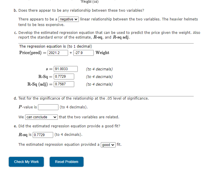
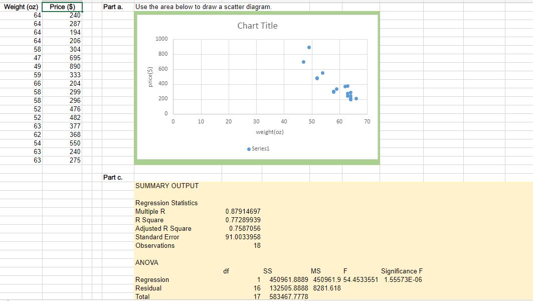
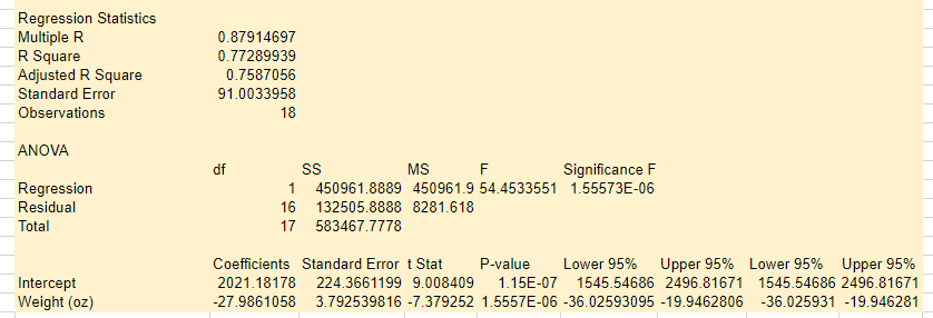
b. Does there appear to be any relationship between these two variables? There appears to be a linear relationship between the two variables. The heavier helmets tend to be less expensive. c. Develop the estimated regression equation that can be used to predict the price given the weight. Also report the standard error of the estimate, R-sq, and R-sq adj . The regression equation is (to 1 decimal) Price ( pred )= Weight s=RSqRSq(adj)(to4decima/s)==(to4decima/s)(to4decima/s) d. Test for the significance of the relationship at the .05 level of significance. P-value is (to 4 decimals). We that the two variables are related. e. Did the estimated regression equation provide a good fit? R-sq is (to 4 decimals). The estimated regression equation provided a fit. Use the area below to draw a scatter diagram. Part c. SUMMARY OUTPUT RegressionStatisticsMultipleRRSquareAdjustedRSquareStandardErrorObservations0.879146970.772899390.758705691.003395818 ANOVA - Series1 RegressionStatisticsMultipleRRSquareAdjustedRSquareStandardErrorObservations0.879146970.772899390.758705691.003395818 ANOVA \begin{tabular}{llrrlrr} & df & \multicolumn{2}{c}{ SS } & MS & F & Significance F \\ Regression & & 1 & 450961.8889 & 450961.9 & 54.4533551 & 1.55573E06 \\ Residual & & 16 & 132505.8888 & 8281.618 & & \\ Total & & 17 & 583467.7778 & & \end{tabular} InterceptWeight(oz)Coefficients2021.1817827.9861058StandardErrortStat224.36611993.792539816P-value9.0084097.379252Lower95%1.15E071.5557E06Upper95%1545.5468636.02593095Lower95%2496.8167119.9462806Upper95%1545.5468636.0259312496.8167119.946281 b. Does there appear to be any relationship between these two variables? There appears to be a linear relationship between the two variables. The heavier helmets tend to be less expensive. c. Develop the estimated regression equation that can be used to predict the price given the weight. Also report the standard error of the estimate, R-sq, and R-sq adj . The regression equation is (to 1 decimal) Price ( pred )= Weight s=RSqRSq(adj)(to4decima/s)==(to4decima/s)(to4decima/s) d. Test for the significance of the relationship at the .05 level of significance. P-value is (to 4 decimals). We that the two variables are related. e. Did the estimated regression equation provide a good fit? R-sq is (to 4 decimals). The estimated regression equation provided a fit. Use the area below to draw a scatter diagram. Part c. SUMMARY OUTPUT RegressionStatisticsMultipleRRSquareAdjustedRSquareStandardErrorObservations0.879146970.772899390.758705691.003395818 ANOVA - Series1 RegressionStatisticsMultipleRRSquareAdjustedRSquareStandardErrorObservations0.879146970.772899390.758705691.003395818 ANOVA \begin{tabular}{llrrlrr} & df & \multicolumn{2}{c}{ SS } & MS & F & Significance F \\ Regression & & 1 & 450961.8889 & 450961.9 & 54.4533551 & 1.55573E06 \\ Residual & & 16 & 132505.8888 & 8281.618 & & \\ Total & & 17 & 583467.7778 & & \end{tabular} InterceptWeight(oz)Coefficients2021.1817827.9861058StandardErrortStat224.36611993.792539816P-value9.0084097.379252Lower95%1.15E071.5557E06Upper95%1545.5468636.02593095Lower95%2496.8167119.9462806Upper95%1545.5468636.0259312496.8167119.946281