Below is an example of a diffusion problem (file Diffusion_Ex). You need to attach your code in Python / Matlab.

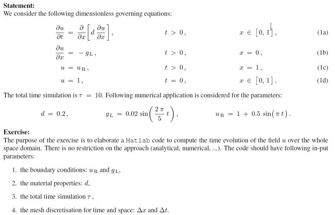
Statement: We consider the following dimensionless governing equations: au at = a ax au d t> 0 [0,1], (la) au = - IL t> 0, x = 0, (lb) ac u = UR, t > 0 x = 1. (10) u = 1, t = 0, 3 6 [0, 1]. (10) The total time simulation is t = 10. Following numerical application is considered for the parameters: d = 0.2, 9L = 0.02 sin (**); 27 5 ur = 1 + 0.5 sin(at). Exercise: The purpose of the exercise is to elaborate a Matlab de to compute the tim olution of the field u over the whol space domain. There is no restriction on the approach (analytical, numerical, ...). The code should have following in-put parameters: 1. the boundary conditions: UR and 9L, 2. the material properties: d, 3. the total time simulation T, 4. the mesh discretisation for time and space: Ax and At. Statement: We consider the following dimensionless governing equations: au at = a ax au d t> 0 [0,1], (la) au = - IL t> 0, x = 0, (lb) ac u = UR, t > 0 x = 1. (10) u = 1, t = 0, 3 6 [0, 1]. (10) The total time simulation is t = 10. Following numerical application is considered for the parameters: d = 0.2, 9L = 0.02 sin (**); 27 5 ur = 1 + 0.5 sin(at). Exercise: The purpose of the exercise is to elaborate a Matlab de to compute the tim olution of the field u over the whol space domain. There is no restriction on the approach (analytical, numerical, ...). The code should have following in-put parameters: 1. the boundary conditions: UR and 9L, 2. the material properties: d, 3. the total time simulation T, 4. the mesh discretisation for time and space: Ax and At