Both Figure 4.8 and table 4.7 had been updated Please CLICK INTO THE QUESTION !!

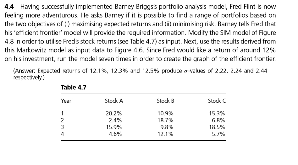
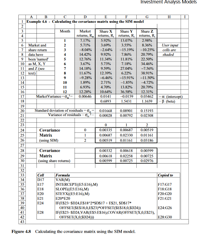
4.4 Having successfully implemented Barney Briggs's portfolio analysis model, Fred Flint is now feeling more adventurous. He asks Barney if it is possible to find a range of portfolios based on the two objectives of (i) maximising expected returns and (ii) minimising risk. Barney tells Fred that his 'efficient frontier' model will provide the required information. Modify the SIM model of Figure 4.8 in order to utilise Fred's stock returns (see Table 4.7) as input. Next, use the results derived from this Markowitz model as input data to Figure 4.6. Since Fred would like a return of around 12% on his investment, run the model seven times in order to create the graph of the efficient frontier (Answer: Expected returns of 12.1%, 12.3% and 12.5% produce -values of 2.22, 2.24 and 2.44 respectively.) Table 4.7 Year Stock A Stock B Stock C 202% 2.4% 15.9% 45% 10.9% 18.7% 92% 12.1% 15.3% 62% 18.5% 57% 4 Investment Analysis Models 1 Example 4.6 - Calculating the covariance matrix using the SIM model Month Market Share X Share YShare Z returns, Rm 7.17% 5.71% -8.04% returns, R. | retums, R. | returns, R. 13.07% 3.55% 4 5.92% 3.69% | 2.98% 8.36% 6Market and 7 sharc return 8 data have 9bccn 'named 10 as M, X, Y 2.64% | - 9.92% 15.19% | -10.25% cells are shaded 7.86% | 20.79% 12.76% 11.34% | 11.81% | 22.50% 71 8% | 34.46% | -7.56% | 6.22% | 38.91% 14.42% 3.67% 14.18% 11 .67% -9.28% 1.89% 6.93% 5.73% 9.59% 12.39% -6.46% 2.71% 4.70% and Z (see 12 text | 27.04% | -15.91%| -11.50% -1.85% | -4.72% 13.82% | 20.79% 12.28% 10.64% | 36.58% | 12.31% -0.0159 0.03462 Market Variance- 0.006460.0141 inte 18 0.6893 1.5431 1.1659 B (beta) ation of residuals 0.01668 0.08900.15 ariance o 0.00028 0.00792 0.02308 23 24 Covariance Matrix using SIM 0.00335 0.00687 0.00519 0.00687 0.02330 0.01161 0.00519 0.01161 0.03186 27 Covariance Matrix (using share returns) 0.00332 0.00618 0.00599 0.00618 0.02258 0.00725 0.00599 0.00725 0.02976 32 Cell D17 E17 E18 ormnla VAR(M) F17:G17 F18:G18 F20:G20 F21:G21 35 INTERCEPT(ES:E16),M) SLOPE((ES:E16),M) 37 STEYX(ES:E16),M) E20* E20 E21 IF(E$23 SD24,ES18 2 SD$17 E$21, SDS17* OFFSET SES18,0,E$23)*OFFSETSES18,0,SD24)) E24:G26 IF(ES23 SD24,VAR(ESS:ES16),COVAR(OFFSET(X,0,E$23), E28:G30 42 43 OFFSET(X,0,SD24 Figure 4.8 Calculating the covariance matrix using the SIM model 4.4 Having successfully implemented Barney Briggs's portfolio analysis model, Fred Flint is now feeling more adventurous. He asks Barney if it is possible to find a range of portfolios based on the two objectives of (i) maximising expected returns and (ii) minimising risk. Barney tells Fred that his 'efficient frontier' model will provide the required information. Modify the SIM model of Figure 4.8 in order to utilise Fred's stock returns (see Table 4.7) as input. Next, use the results derived from this Markowitz model as input data to Figure 4.6. Since Fred would like a return of around 12% on his investment, run the model seven times in order to create the graph of the efficient frontier (Answer: Expected returns of 12.1%, 12.3% and 12.5% produce -values of 2.22, 2.24 and 2.44 respectively.) Table 4.7 Year Stock A Stock B Stock C 202% 2.4% 15.9% 45% 10.9% 18.7% 92% 12.1% 15.3% 62% 18.5% 57% 4 Investment Analysis Models 1 Example 4.6 - Calculating the covariance matrix using the SIM model Month Market Share X Share YShare Z returns, Rm 7.17% 5.71% -8.04% returns, R. | retums, R. | returns, R. 13.07% 3.55% 4 5.92% 3.69% | 2.98% 8.36% 6Market and 7 sharc return 8 data have 9bccn 'named 10 as M, X, Y 2.64% | - 9.92% 15.19% | -10.25% cells are shaded 7.86% | 20.79% 12.76% 11.34% | 11.81% | 22.50% 71 8% | 34.46% | -7.56% | 6.22% | 38.91% 14.42% 3.67% 14.18% 11 .67% -9.28% 1.89% 6.93% 5.73% 9.59% 12.39% -6.46% 2.71% 4.70% and Z (see 12 text | 27.04% | -15.91%| -11.50% -1.85% | -4.72% 13.82% | 20.79% 12.28% 10.64% | 36.58% | 12.31% -0.0159 0.03462 Market Variance- 0.006460.0141 inte 18 0.6893 1.5431 1.1659 B (beta) ation of residuals 0.01668 0.08900.15 ariance o 0.00028 0.00792 0.02308 23 24 Covariance Matrix using SIM 0.00335 0.00687 0.00519 0.00687 0.02330 0.01161 0.00519 0.01161 0.03186 27 Covariance Matrix (using share returns) 0.00332 0.00618 0.00599 0.00618 0.02258 0.00725 0.00599 0.00725 0.02976 32 Cell D17 E17 E18 ormnla VAR(M) F17:G17 F18:G18 F20:G20 F21:G21 35 INTERCEPT(ES:E16),M) SLOPE((ES:E16),M) 37 STEYX(ES:E16),M) E20* E20 E21 IF(E$23 SD24,ES18 2 SD$17 E$21, SDS17* OFFSET SES18,0,E$23)*OFFSETSES18,0,SD24)) E24:G26 IF(ES23 SD24,VAR(ESS:ES16),COVAR(OFFSET(X,0,E$23), E28:G30 42 43 OFFSET(X,0,SD24 Figure 4.8 Calculating the covariance matrix using the SIM model