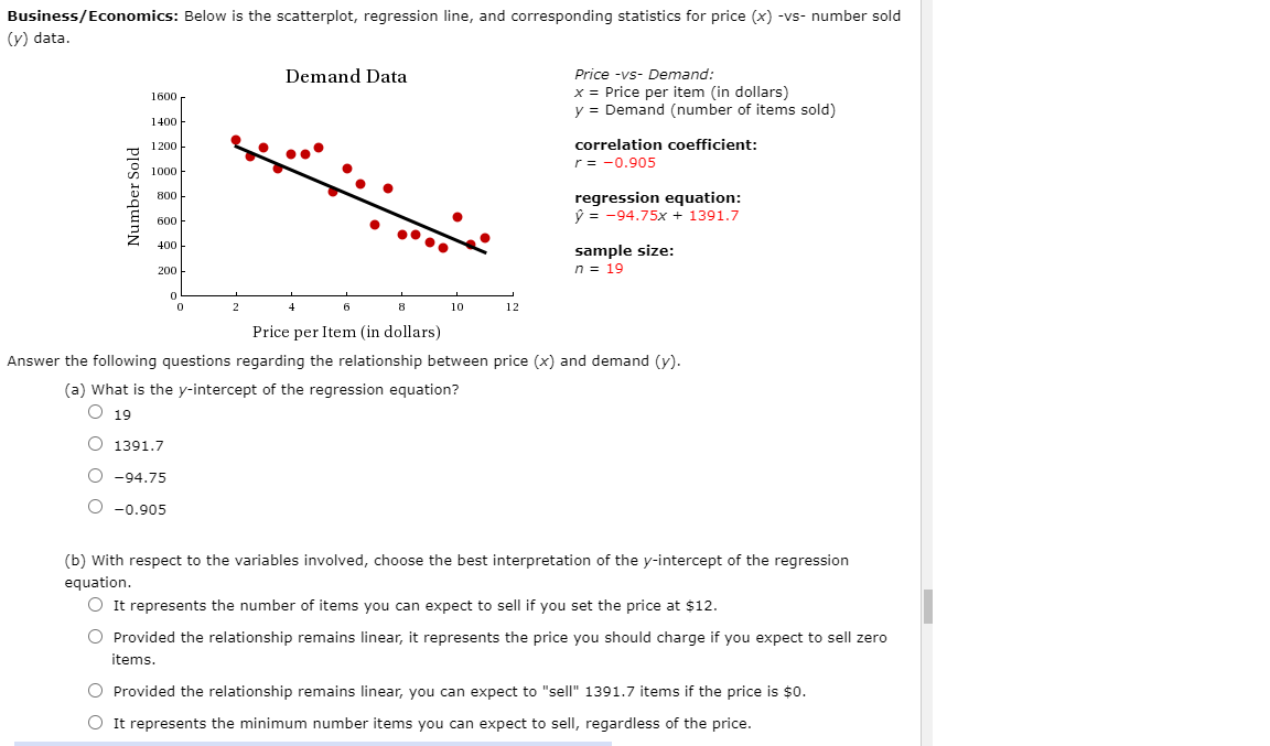
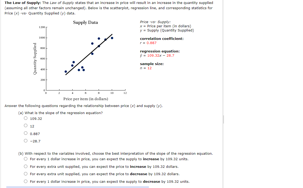
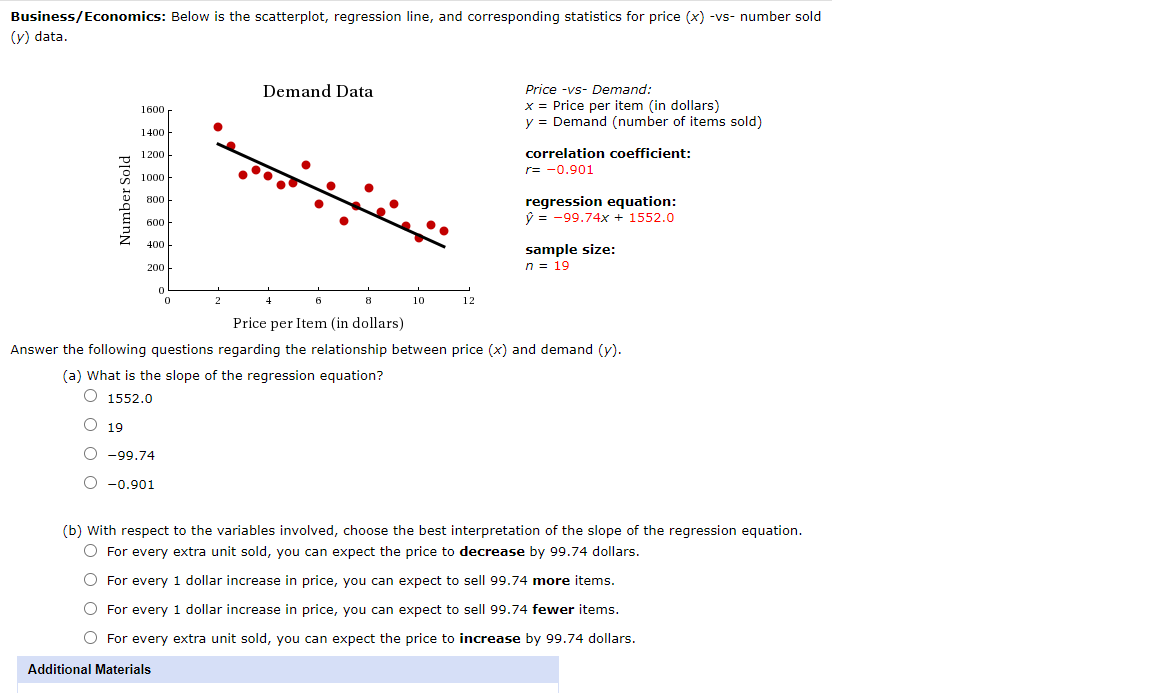
Business/Economics: Below is the scatterplot, regression line, and corresponding statistics for price (x) -vs- number sold (y) data. Demand Data Price -VS- Demand: 1500 x = Price per item (in dollars) y 2 Demand (number of items sold) 1400 E 1200 . ... :rregagtggn ooefcmnt. '2 1000 ' I1 B 500 regression equation: E m p = 94.75x + 1391.7 :1 Z . 40 sample Size: 200 n = 19 o . . . . . . u 2 a a a 10 12 Price perltem (in dollars) Answer the following questions regarding the relationship between price (x) and demand (y). (a) What is the y-intercept of the regression equation? 0 19 1391.7 94.75 000 D.905 (b) with respect to the variables involved, choose the best interpretation of the yintercept of the regression equation. 0 It represents the number of items you can expect to sell if you set the price at $12. 0 Provided the relationship remains linear, it represents the price you should charge if you expect to sell zero items. 0 Provided the relationship remains linear, you can expect to "sell" 1391.]Ir items if the price is $0. 0 It represents the minimum number items you can expect to sell, regardless of the price. The Law of Supply: The Law ofSuppl'y states that an increase in price will result in an increase in the quantity supplied (assuming all other factors remain unchanged). Below is the scatterplot, regression line, and corresponding statistics for Price (x) -vs- Quantity Supplied (y) data. Supply Data Price vs Supply: 1200 x = Price per item (in dollars} y = Supply (Quantity Supplied} 1000 correlation coefcient: "U r = 0.887 U : aoo & regression equation: a y = 109.32X 28.7 500 E - E- sample Size: n, 400 n = 12 :s O' 200 o . . . . . . o 2 4 s a 10 12 Price per item (in dollars) Answer the following questions regarding the relationship between price (x) and supply 0/). (a) What is the slope of the regression equation? 0 109.32 12 0.887 000 28.7 (b) with respect to the variables involved, choose the best interpretation of the slope of the regression equation. 0 For every 1 dollar increase in price, you can expect the supply to increase by 109.32 units. 0 For every extra unit supplied, you can expect the price to increase by 109.32 dollars. 0 For every extra unit supplied, you can expect the price to decrease by 109.32 dollars. 0 For every 1 dollar increase in price, you can expect the supply to decrease by 109.32 units. Business/Economics: Below is the scatterplot, regression line, and corresponding statistics for price (x) -vs- number sold (y) data. Demand Data Price -vs- Demand: 1600 x = Price per item (in dollars) 1400 y = Demand (number of items sold) Number Sold 1200 correlation coefficient: 1000 = -0.901 800 regression equation: 600 = -99.74x + 1552.0 400 sample size: 200 n = 19 2 8 10 12 Price per Item (in dollars) Answer the following questions regarding the relationship between price (x) and demand (y). (a) What is the slope of the regression equation? 1552.0 O 19 O -99.74 O -0.901 (b) With respect to the variables involved, choose the best interpretation of the slope of the regression equation. For every extra unit sold, you can expect the price to decrease by 99.74 dollars. O For every 1 dollar increase in price, you can expect to sell 99.74 more items. O For every 1 dollar increase in price, you can expect to sell 99.74 fewer items. For every extra unit sold, you can expect the price to increase by 99.74 dollars. Additional Materials