$($C$)$ Modelling Report $(50\%)$

Aim

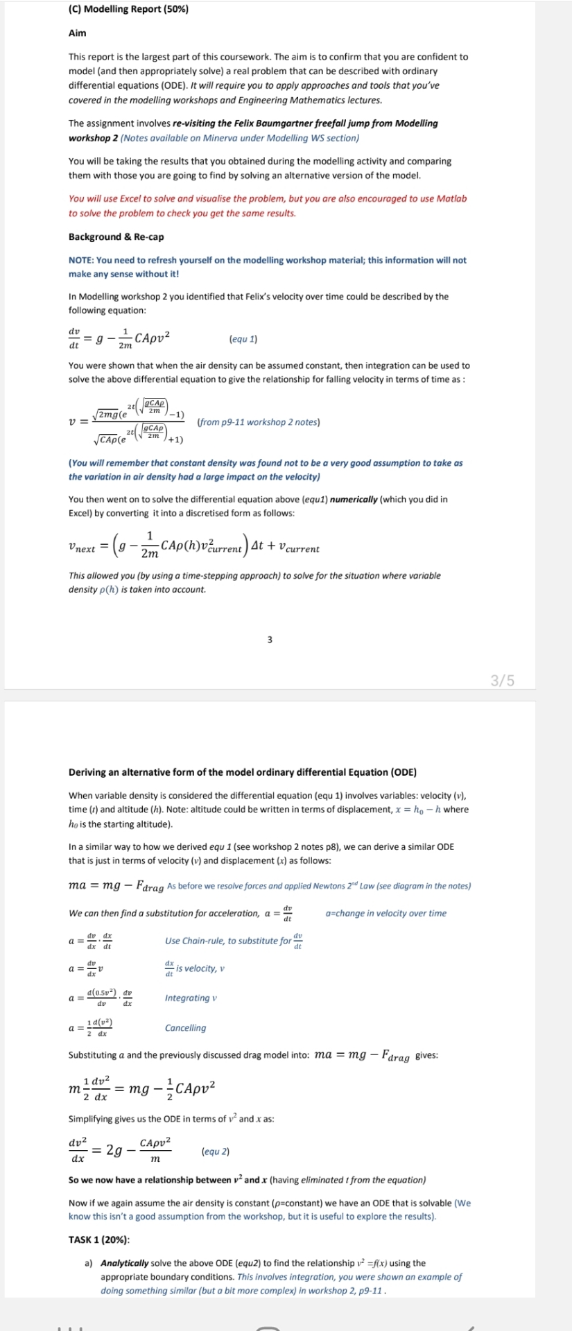
This report is the largest part of this coursework. The aim is to confirm that you are confident to model $($and then appropriately solve$)$ a real problem that can be described with ordinary differential equations $($ODE$).$ It will require you to apply approaches and tools that you've covered in the modelling workshops and Engineering Mathematics lectures.

The assignment involves re$-$visiting the Felix Baumgartner freefall jump from Modelling workshop $2($Notes available on Minerva under Modelling WS section$)$

You will be taking the results that you obtained during the modelling activity and comparing them with those you are going to find by solving an alternative version of the model.

You will use Excel to solve and visualise the problem, but you are also encouraged to use Matlab to solve the problem to check you get the same results.

Background & Re$-$cap

NOTE: You need to refresh yourself on the modelling workshop material; this information will not make any sense without it$!$

In Modelling workshop $2$ you identified that Felix's velocity over time could be described by the following equation:

$\frac{dv}{dt}=g-\frac{1}{2m}CA{v}^2,($equ $1)$

You were shown that when the air density can be assumed constant, then integration can be used to solve the above differential equation to give the relationship for falling velocity in terms of time as :

$($from p$9-11$ workshop $2$notes$)$

$($You will remember that constant density was found not to be a very good assumption to take as the variation in air density had a large impact on the velocity$)$

You then went on to solve the differential equation above $($equ$1)$ numerically $($which you did in Excel$)$ by converting it into a discretised form as follows:

$v_{\text{n}\text{e}\text{x}\text{t}}=(g-\frac{1}{2m}CA(h)v_{\text{c}\text{u}\text{r}\text{r}\text{e}\text{n}\text{t}}^2)t+v_{\text{c}\text{u}\text{r}\text{r}\text{e}\text{n}\text{t}}$

This allowed you $($by using a time$-$stepping approach$)$ to solve for the situation where variable density $(h)$ is taken into account.

$3$

Deriving an alternative form of the model ordinary differential Equation $($ODE$)$

When variable density is considered the differential equation $($equ $1)$ involves variables: velocity $(v),$ time $(t)$ and altitude $(h).$ Note: altitude could be written in terms of displacement, $x=h_0-h$ where $h_0$ is the starting altitude$).$

In a similar way to how we derived equ $1($see workshop $2$ notes p $8),$ we can derive a similar ODE that is just in terms of velocity $(v)$ and displacement $(x)$ as follows:

$ma=mg-F_{\text{d}\text{r}\text{a}\text{g}}$ As before we resolve forces and applied Newtons $2^{nd}$ Law $($see diagram in the notes$)$

We can then find a substitution for acceleration, $a=\frac{dv}{dt},a=$change in velocity over time

$a=\frac{dv}{dx}*\frac{dx}{dt},$ Use Chain$-$rule, to substitute for $\frac{dv}{dt}$

$a=\frac{dv}{dx}v,\frac{dx}{dt}$ is velocity, $v$

$a=\frac{d(0\mathrm{.}5v^2)}{dv}*\frac{dv}{dx},$ Integrating $v$

$a=\frac{1}{2}\frac{d(v^2)}{dx},$ Cancelling

Substituting a and the previously discussed drag model into: $ma=mg-F_{\text{d}\text{r}\text{a}\text{g}}$ gives:

$m\frac{1}{2}\frac{d{v}^2}{dx}=mg-\frac{1}{2}CA{v}^2$

Simplifying gives us the ODE in terms of $v^2$ and $x$ as:

$\frac{d{v}^2}{dx}=2g-\frac{CA{v}^2}{m},(equ2)$

So we now have a relationship between $v^2$ and $x($having eliminated $t$ from the equation$)$

Now if we again assume the air density is constant $(=$ constant$)$ we have an ODE that is solvable $($We know this isn't a good assumption from the workshop, but it is useful to explore the results$).$

TASK $1(20\%)$:

a$)$ Analytically solve the above ODE $($equ$2)$ to find the relationship $v^2=f(x)$ using the appropriate boundary conditions. This involves integration, you were shown an example of doing something similar $($but a bit more complex$)$ in workshop $2,$ p$9-11.$