Can I get the python programs for each of these computational physics problems?

Textbooks for reference:

? "Computational Physics" by Mark Newman (guide to Python in computational physics)

? "Numerical Recipes" by W. H. Press et al. (covers very comprehensibly a vast range of numerical topics; 3rd edition is in C++; older editions, e.g. in C, are freely available online)

? "Clean Code" by Robert C. Martin (great book on good programming practices)

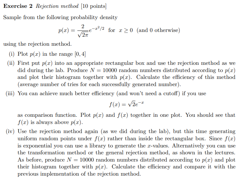
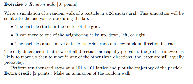
Exercise 2 Rejection method [10 points] Sample from the following probability density 2 2 e sasatfh g | d 0 otherwis T e or and 0 otherwise plx) o = ( ) using the rejection method. (i) Plot p(x) in the range [0, 4] (ii) First put p(x) into an appropriate rectangular box and use the rejection method as we did during the lab. Produce N = 10000 random numbers distributed according to p(z) and plot their histogram together with p(x). Calculate the efficiency of this method (average number of tries for each successfully generated number). (iii) You can achieve much better efficiency (and won't need a cutoff) if you use f(z)=v2e" as comparison function. Plot p(x) and f(x) together in one plot. You should see that f(x) is always above p(x). (iv) Use the rejection method again (as we did during the lab), but this time generating uniform random points under f(z) rather than inside the rectangular box. Since f(z) is exponential you can use a library to generate the xz-values. Alternatively you can use the transformation method or the general rejection method, as shown in the lectures. As before, produce N = 10000 random numbers distributed according to p(x) and plot their histogram together with p(x). Calculate the efficiency and compare it with the previous implementation of the rejection method. Exercise 3 Random walk [10 points] Write a simulation of a random walk of a particle in a 2d square grid. This simulation will be similar to the one you wrote during the lab: e The particle starts in the center of the grid. e [t can move to one of the neighboring cells: up, down, left, or right. e The particle cannot move outside the grid: choose a new random direction instead. The only difference is that now not all directions are equally probable: the particle is twice as likely to move up than to move in any of the other three directions (the latter are still equally probable). Perform ten thousand steps on a 101 x 101 lattice and plot the trajectory of the particle. Extra credit [5 points|: Make an animation of the random walk