Can some one help me I know how to do some of it just not all of it. ASAP please.

can someone help without charging extra. im already paying to use the this site.

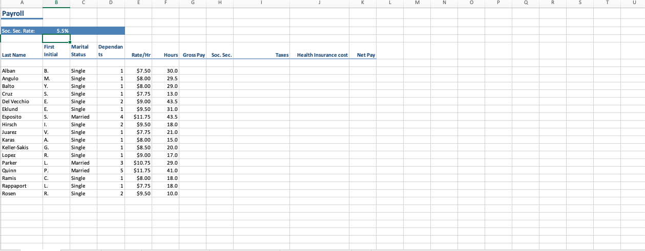
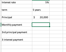
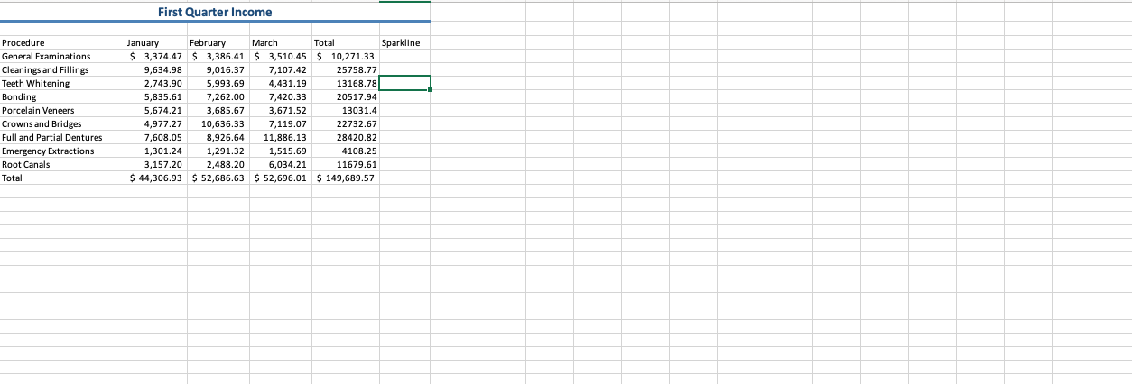
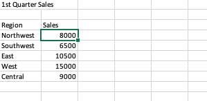
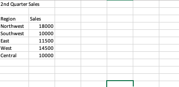
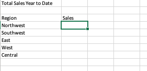
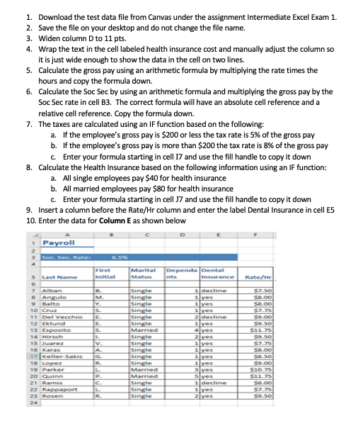
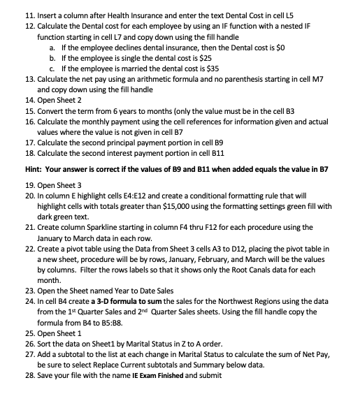
Interest rate 5% term 5 years Principal $20,000 Monthly payment 3rd principal payment 3 interest payment First Quarter Income \begin{tabular}{|l|r|r|r|r|r|} \hline Procedure & \multicolumn{1}{|l|}{ January } & \multicolumn{1}{|l|}{ February } & \multicolumn{1}{|l|}{ March } & \multicolumn{1}{|l|}{ Total } & Sparkline \\ \hline General Examinations & $3,374.47 & $3,386.41 & $3,510.45 & $10,271.33 & \\ \hline Cleanings and Fillings & 9,634.98 & 9,016.37 & 7,107.42 & 25758.77 & \\ \hline Teeth Whitening & 2,743.90 & 5,993.69 & 4,431.19 & 13168.78 & \\ \hline Bonding & 5,835.61 & 7,262.00 & 7,420.33 & 20517.94 & \\ \hline Porcelain Veneers & 5,674.21 & 3,685.67 & 3,671.52 & 13031.4 & \\ \hline Crowns and Bridges & 4,977.27 & 10,636.33 & 7,119.07 & 22732.67 & \\ \hline Full and Partial Dentures & 7,608.05 & 8,926.64 & 11,886.13 & 28420.82 & \\ \hline Emergency Extractions & 1,301.24 & 1,291.32 & 1,515.69 & 4108.25 & \\ Root Canals & 3,157.20 & 2,488.20 & 6,034.21 & 11679.61 & \\ \hline Total & $44,306.93 & $52,686.63 & $52,696.01 & $149,689.57 & \\ \hline \end{tabular} 1st Quarter Sales \begin{tabular}{|r|r|} \hline Region & \multicolumn{1}{|l|}{ Sales } \\ \hline Northwest & 8000 \\ \hline Southwest & 6500 \\ \hline East & 10500 \\ \hline West & 15000 \\ \hline Central & 9000 \\ \hline \end{tabular} 2nd Quarter Sales \begin{tabular}{l|r} \hline Region & \multicolumn{1}{|l}{ Sales } \\ \hline Northwest & 18000 \\ \hline Southwest & 10000 \\ \hline East & 11500 \\ \hline West & 14500 \\ \hline Central & 10000 \\ \hline \end{tabular} Total Sales Year to Date \begin{tabular}{|l|l|} \hline Region & \multicolumn{1}{|l|}{ Sales } \\ \hline Northwest & \\ \hline Southwest & \\ \hline East & \\ \hline West & \\ \hline Central & \\ \hline \end{tabular} 1. Download the test data file from Canvas under the assignment Intermediate Excel Exam 1. 2. Save the file on your desktop and do not change the file name. 3. Widen column D to 11 pts. 4. Wrap the text in the cell labeled health insurance cost and manually adjust the column so it is just wide enough to show the data in the cell on two lines. 5. Calculate the gross pay using an arithmetic formula by multiplying the rate times the hours and copy the formula down. 6. Calculate the Soc Sec by using an arithmetic formula and multiplying the gross pay by the Soc Sec rate in cell B3. The correct formula will have an absolute cell reference and a relative cell reference. Copy the formula down. 7. The taxes are calculated using an IF function based on the following: a. If the employee's gross pay is $200 or less the tax rate is 5% of the gross pay b. If the employee's gross pay is more than $200 the tax rate is 8% of the gross pay c. Enter your formula starting in cell 17 and use the fill handle to copy it down 8. Calculate the Health Insurance based on the following information using an IF function: a. All single employees pay $40 for health insurance b. All married employees pay $80 for health insurance c. Enter your formula starting in cell J7 and use the fill handle to copy it down 9. Insert a column before the Rate/Hr column and enter the label Dental Insurance in cell E5 11. Insert a column after Health Insurance and enter the text Dental Cost in cell L5 12. Calculate the Dental cost for each employee by using an IF function with a nested IF function starting in cell L7 and copy down using the fill handle a. If the employee declines dental insurance, then the Dental cost is $0 b. If the employee is single the dental cost is $25 c. If the employee is married the dental cost is $35 13. Calculate the net pay using an arithmetic formula and no parenthesis starting in cell M7 and copy down using the fill handle 14. Open Sheet 2 15. Convert the term from 6 years to months (only the value must be in the cell B3 16. Calculate the monthly payment using the cell references for information given and actual values where the value is not given in cell B7 17. Calculate the second principal payment portion in cell B9 18. Calculate the second interest payment portion in cell B11 Hint: Your answer is correct if the values of B9 and B11 when added equals the value in B7 19. Open Sheet 3 20. In column E highlight cells E4:E12 and create a conditional formatting rule that will highlight cells with totals greater than $15,000 using the formatting settings green fill with dark green text. 21. Create column Sparkline starting in column F4 thru F12 for each procedure using the January to March data in each row. 22. Create a pivot table using the Data from Sheet 3 cells A3 to D12, placing the pivot table in a new sheet, procedure will be by rows, January, February, and March will be the values by columns. Filter the rows labels so that it shows only the Root Canals data for each month. 23. Open the Sheet named Year to Date Sales 24. In cell B4 create a 3-D formula to sum the sales for the Northwest Regions using the data from the 1st Quarter Sales and 2nd Quarter Sales sheets. Using the fill handle copy the formula from B4 to B5B8. 25. Open Sheet 1 26. Sort the data on Sheet 1 by Marital Status in Z to A order. 27. Add a subtotal to the list at each change in Marital Status to calculate the sum of Net Pay, be sure to select Replace Current subtotals and Summary below data. 28. Save your file with the name IE Exam Finished and submit Interest rate 5% term 5 years Principal $20,000 Monthly payment 3rd principal payment 3 interest payment First Quarter Income \begin{tabular}{|l|r|r|r|r|r|} \hline Procedure & \multicolumn{1}{|l|}{ January } & \multicolumn{1}{|l|}{ February } & \multicolumn{1}{|l|}{ March } & \multicolumn{1}{|l|}{ Total } & Sparkline \\ \hline General Examinations & $3,374.47 & $3,386.41 & $3,510.45 & $10,271.33 & \\ \hline Cleanings and Fillings & 9,634.98 & 9,016.37 & 7,107.42 & 25758.77 & \\ \hline Teeth Whitening & 2,743.90 & 5,993.69 & 4,431.19 & 13168.78 & \\ \hline Bonding & 5,835.61 & 7,262.00 & 7,420.33 & 20517.94 & \\ \hline Porcelain Veneers & 5,674.21 & 3,685.67 & 3,671.52 & 13031.4 & \\ \hline Crowns and Bridges & 4,977.27 & 10,636.33 & 7,119.07 & 22732.67 & \\ \hline Full and Partial Dentures & 7,608.05 & 8,926.64 & 11,886.13 & 28420.82 & \\ \hline Emergency Extractions & 1,301.24 & 1,291.32 & 1,515.69 & 4108.25 & \\ Root Canals & 3,157.20 & 2,488.20 & 6,034.21 & 11679.61 & \\ \hline Total & $44,306.93 & $52,686.63 & $52,696.01 & $149,689.57 & \\ \hline \end{tabular} 1st Quarter Sales \begin{tabular}{|r|r|} \hline Region & \multicolumn{1}{|l|}{ Sales } \\ \hline Northwest & 8000 \\ \hline Southwest & 6500 \\ \hline East & 10500 \\ \hline West & 15000 \\ \hline Central & 9000 \\ \hline \end{tabular} 2nd Quarter Sales \begin{tabular}{l|r} \hline Region & \multicolumn{1}{|l}{ Sales } \\ \hline Northwest & 18000 \\ \hline Southwest & 10000 \\ \hline East & 11500 \\ \hline West & 14500 \\ \hline Central & 10000 \\ \hline \end{tabular} Total Sales Year to Date \begin{tabular}{|l|l|} \hline Region & \multicolumn{1}{|l|}{ Sales } \\ \hline Northwest & \\ \hline Southwest & \\ \hline East & \\ \hline West & \\ \hline Central & \\ \hline \end{tabular} 1. Download the test data file from Canvas under the assignment Intermediate Excel Exam 1. 2. Save the file on your desktop and do not change the file name. 3. Widen column D to 11 pts. 4. Wrap the text in the cell labeled health insurance cost and manually adjust the column so it is just wide enough to show the data in the cell on two lines. 5. Calculate the gross pay using an arithmetic formula by multiplying the rate times the hours and copy the formula down. 6. Calculate the Soc Sec by using an arithmetic formula and multiplying the gross pay by the Soc Sec rate in cell B3. The correct formula will have an absolute cell reference and a relative cell reference. Copy the formula down. 7. The taxes are calculated using an IF function based on the following: a. If the employee's gross pay is $200 or less the tax rate is 5% of the gross pay b. If the employee's gross pay is more than $200 the tax rate is 8% of the gross pay c. Enter your formula starting in cell 17 and use the fill handle to copy it down 8. Calculate the Health Insurance based on the following information using an IF function: a. All single employees pay $40 for health insurance b. All married employees pay $80 for health insurance c. Enter your formula starting in cell J7 and use the fill handle to copy it down 9. Insert a column before the Rate/Hr column and enter the label Dental Insurance in cell E5 11. Insert a column after Health Insurance and enter the text Dental Cost in cell L5 12. Calculate the Dental cost for each employee by using an IF function with a nested IF function starting in cell L7 and copy down using the fill handle a. If the employee declines dental insurance, then the Dental cost is $0 b. If the employee is single the dental cost is $25 c. If the employee is married the dental cost is $35 13. Calculate the net pay using an arithmetic formula and no parenthesis starting in cell M7 and copy down using the fill handle 14. Open Sheet 2 15. Convert the term from 6 years to months (only the value must be in the cell B3 16. Calculate the monthly payment using the cell references for information given and actual values where the value is not given in cell B7 17. Calculate the second principal payment portion in cell B9 18. Calculate the second interest payment portion in cell B11 Hint: Your answer is correct if the values of B9 and B11 when added equals the value in B7 19. Open Sheet 3 20. In column E highlight cells E4:E12 and create a conditional formatting rule that will highlight cells with totals greater than $15,000 using the formatting settings green fill with dark green text. 21. Create column Sparkline starting in column F4 thru F12 for each procedure using the January to March data in each row. 22. Create a pivot table using the Data from Sheet 3 cells A3 to D12, placing the pivot table in a new sheet, procedure will be by rows, January, February, and March will be the values by columns. Filter the rows labels so that it shows only the Root Canals data for each month. 23. Open the Sheet named Year to Date Sales 24. In cell B4 create a 3-D formula to sum the sales for the Northwest Regions using the data from the 1st Quarter Sales and 2nd Quarter Sales sheets. Using the fill handle copy the formula from B4 to B5B8. 25. Open Sheet 1 26. Sort the data on Sheet 1 by Marital Status in Z to A order. 27. Add a subtotal to the list at each change in Marital Status to calculate the sum of Net Pay, be sure to select Replace Current subtotals and Summary below data. 28. Save your file with the name IE Exam Finished and submit