Can someone please help with this problem.. Can you please show step by step in pictures to see if it's correct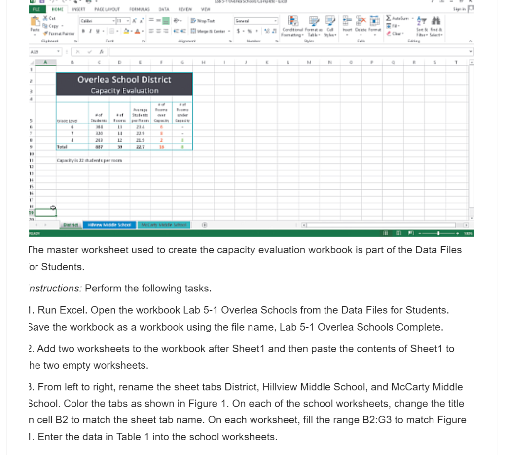

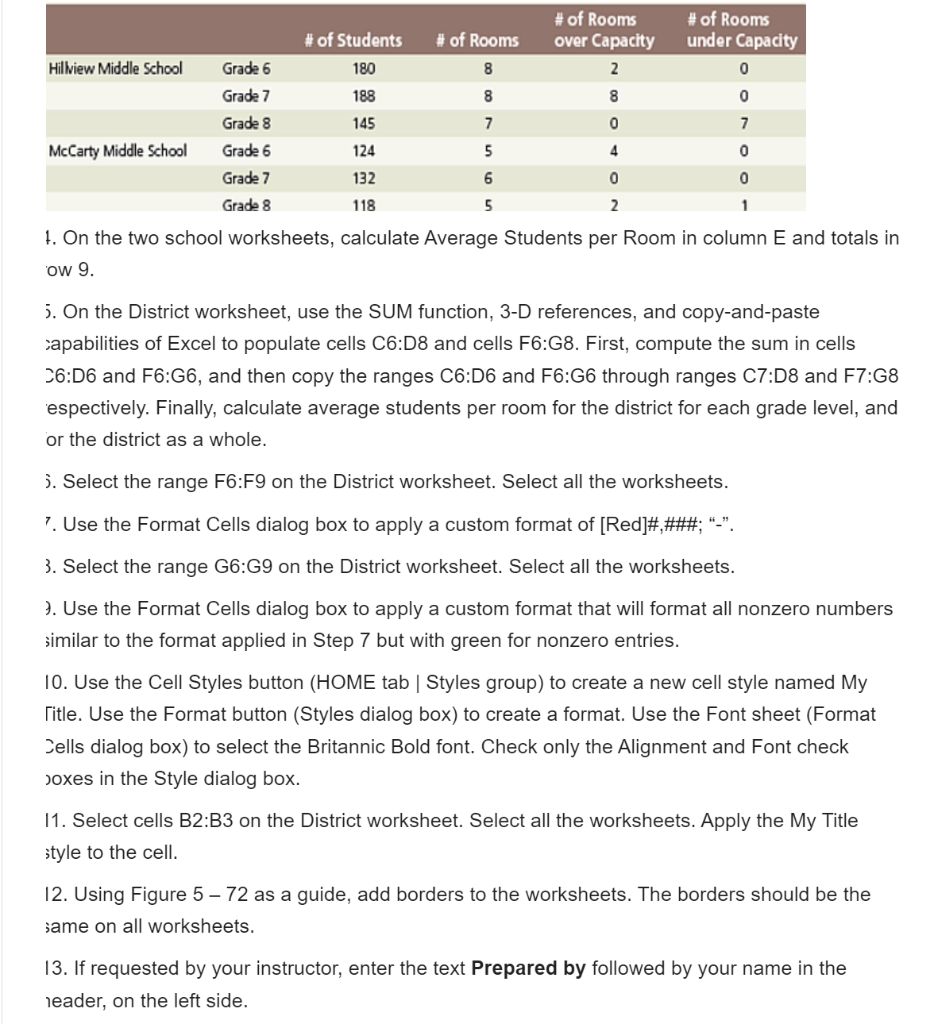
Deftaschscored FLE HOMI WAT PAGE LAYOUT TOIMULAS DATA EN Sky X Cut CHRY - 11 27 # CA Cute Cc - ... Contos For Table Cu AIS . M $ T . 2 Overlea School District Capacity Evaluation 3 4 Bu 5 Se . Tert con 214 14 2 233 23 227 18 10 11 Cityisen parem 12 11 14 15 1 19 an ind MER MM Sche WOME The master worksheet used to create the capacity evaluation workbook is part of the Data Files or Students. instructions: Perform the following tasks. 1. Run Excel. Open the workbook Lab 5-1 Overlea Schools from the Data Files for Students. Save the workbook as a workbook using the file name, Lab 5-1 Overlea Schools Complete. 2. Add two worksheets to the workbook after Sheet1 and then paste the contents of Sheet1 to he two empty worksheets. 3. From left to right, rename the sheet tabs District, Hillview Middle School, and McCarty Middle School. Color the tabs as shown in Figure 1. On each of the school worksheets, change the title n cell B2 to match the sheet tab name. On each worksheet, fill the range B2:G3 to match Figure 1. Enter the data in Table 1 into the school worksheets. # of Rooms # of Rooms over Capacity 2 # of Students 180 188 # of Rooms under Capacity 0 Hillview Middle School 8 8 8 0 145 7 0 7 Grade 6 Grade 7 Grade 8 Grade 6 Grade 7 Grade 8 McCarty Middle School 124 5 4 0 132 6 0 0 118 5 2 1 1. On the two school worksheets, calculate Average Students per Room in column E and totals in ow 9. 5. On the District worksheet, use the SUM function, 3-D references, and copy-and-paste capabilities of Excel to populate cells C6:D8 and cells F6:G8. First, compute the sum in cells 26:06 and 76:G6, and then copy the ranges C6:06 and F6:G6 through ranges C7:D8 and F7:G8 espectively. Finally, calculate average students per room for the district for each grade level, and or the district as a whole. 3. Select the range F6:F9 on the District worksheet. Select all the worksheets. 7. Use the Format Cells dialog box to apply a custom format of [Red]#,###; -. 3. Select the range G6:G9 on the District worksheet. Select all the worksheets. 7. Use the Format Cells dialog box to apply a custom format that will format all nonzero numbers similar to the format applied in Step 7 but with green for nonzero entries. 10. Use the Cell Styles button (HOME tab Styles group) to create a new cell style named My Title. Use the Format button (Styles dialog box) to create a format. Use the Font sheet (Format Cells dialog box) to select the Britannic Bold font. Check only the Alignment and Font check boxes in the Style dialog box. 11. Select cells B2:B3 on the District worksheet. Select all the worksheets. Apply the My Title style to the cell. 12. Using Figure 5 72 as a guide, add borders to the worksheets. The borders should be the same on all worksheets. 13. If requested by your instructor, enter the text Prepared by followed by your name in the header, on the left side. Deftaschscored FLE HOMI WAT PAGE LAYOUT TOIMULAS DATA EN Sky X Cut CHRY - 11 27 # CA Cute Cc - ... Contos For Table Cu AIS . M $ T . 2 Overlea School District Capacity Evaluation 3 4 Bu 5 Se . Tert con 214 14 2 233 23 227 18 10 11 Cityisen parem 12 11 14 15 1 19 an ind MER MM Sche WOME The master worksheet used to create the capacity evaluation workbook is part of the Data Files or Students. instructions: Perform the following tasks. 1. Run Excel. Open the workbook Lab 5-1 Overlea Schools from the Data Files for Students. Save the workbook as a workbook using the file name, Lab 5-1 Overlea Schools Complete. 2. Add two worksheets to the workbook after Sheet1 and then paste the contents of Sheet1 to he two empty worksheets. 3. From left to right, rename the sheet tabs District, Hillview Middle School, and McCarty Middle School. Color the tabs as shown in Figure 1. On each of the school worksheets, change the title n cell B2 to match the sheet tab name. On each worksheet, fill the range B2:G3 to match Figure 1. Enter the data in Table 1 into the school worksheets. # of Rooms # of Rooms over Capacity 2 # of Students 180 188 # of Rooms under Capacity 0 Hillview Middle School 8 8 8 0 145 7 0 7 Grade 6 Grade 7 Grade 8 Grade 6 Grade 7 Grade 8 McCarty Middle School 124 5 4 0 132 6 0 0 118 5 2 1 1. On the two school worksheets, calculate Average Students per Room in column E and totals in ow 9. 5. On the District worksheet, use the SUM function, 3-D references, and copy-and-paste capabilities of Excel to populate cells C6:D8 and cells F6:G8. First, compute the sum in cells 26:06 and 76:G6, and then copy the ranges C6:06 and F6:G6 through ranges C7:D8 and F7:G8 espectively. Finally, calculate average students per room for the district for each grade level, and or the district as a whole. 3. Select the range F6:F9 on the District worksheet. Select all the worksheets. 7. Use the Format Cells dialog box to apply a custom format of [Red]#,###; -. 3. Select the range G6:G9 on the District worksheet. Select all the worksheets. 7. Use the Format Cells dialog box to apply a custom format that will format all nonzero numbers similar to the format applied in Step 7 but with green for nonzero entries. 10. Use the Cell Styles button (HOME tab Styles group) to create a new cell style named My Title. Use the Format button (Styles dialog box) to create a format. Use the Font sheet (Format Cells dialog box) to select the Britannic Bold font. Check only the Alignment and Font check boxes in the Style dialog box. 11. Select cells B2:B3 on the District worksheet. Select all the worksheets. Apply the My Title style to the cell. 12. Using Figure 5 72 as a guide, add borders to the worksheets. The borders should be the same on all worksheets. 13. If requested by your instructor, enter the text Prepared by followed by your name in the header, on the left side