Can you construct an efficient frontier for the following model. It has n securities in a portfolio. Please label everything so that I can paste your diagram into my research paper.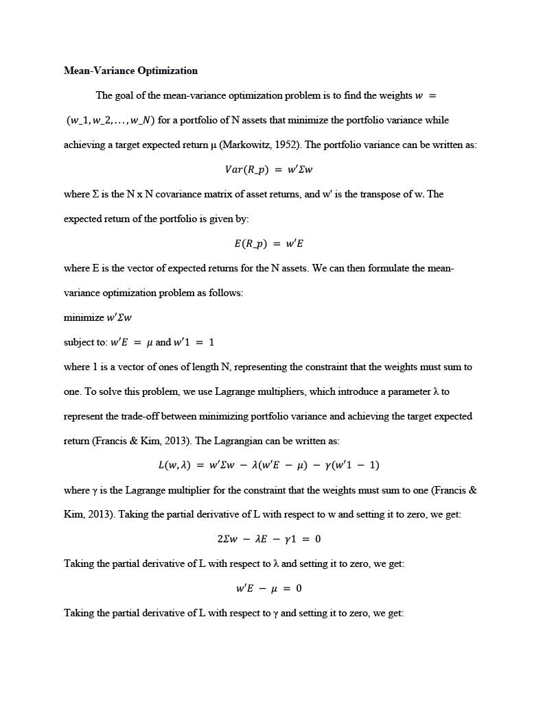

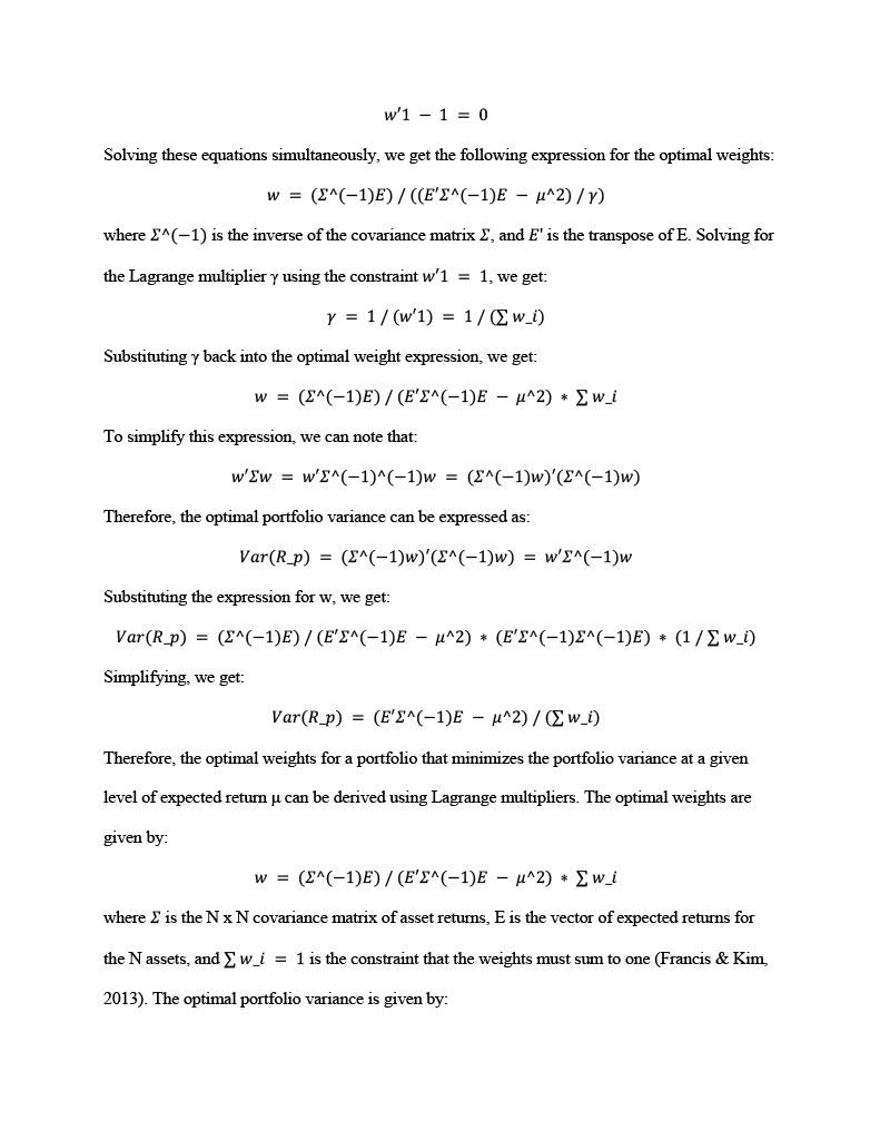
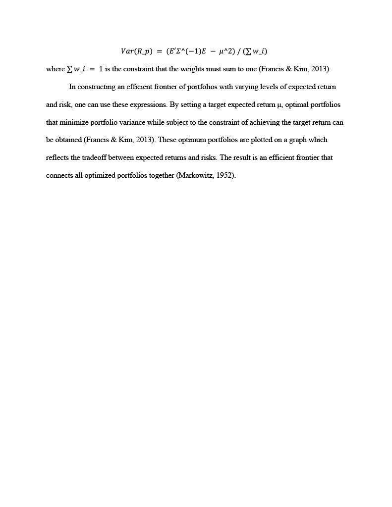
Mean-Variance Optimization The goal of the mean-variance optimization problem is to find the weights w= (w1,w2,,wN) for a portfolio of N assets that minimize the portfolio variance while achieving a target expected return (Markowitz, 1952). The portfolio variance can be written as: Var(R_p)=ww where is the NxN covariance matrix of asset returns, and w' is the transpose of w. The expected return of the portfolio is given by: E(Rp)=wE where E is the vector of expected returns for the N assets. We can then formulate the meanvariance optimization problem as follows: minimizeww subject to: wE= and w1=1 where 1 is a vector of ones of length N, representing the constraint that the weights must sum to one. To solve this problem, we use Lagrange multipliers, which introduce a parameter to represent the trade-off between minimizing portfolio variance and achieving the target expected return (Francis \& Kim, 2013). The Lagrangian can be written as: L(w,)=ww(wE)(w11) where is the Lagrange multiplier for the constraint that the weights must sum to one (Francis \& Kim, 2013). Taking the partial derivative of L with respect to w and setting it to zero, we get: 2wE1=0 Taking the partial derivative of L with respect to and setting it to zero, we get: wE=0 Taking the partial derivative of L with respect to and setting it to zero, we get: w11=0 Solving these equations simultaneously, we get the following expression for the optimal weights: w=((1)E)/((E(1)E2)/) where (1) is the inverse of the covariance matrix , and E is the transpose of E. Solving for the Lagrange multiplier using the constraint w1=1, we get: =1/(w1)=1/(wi) Substituting back into the optimal weight expression, we get: w=((1)E)/(E(1)E2)wi To simplify this expression, we can note that: ww=w(1)(1)w=((1)w)((1)w) Therefore, the optimal portfolio variance can be expressed as: Var(R_p)=((1)w)((1)w)=w(1)w Substituting the expression for w, we get: Var(Rp)=((1)E)/(E(1)E2)(E(1)(1)E)(1/wi) Simplifying, we get: Var(Rp)=(E(1)E2)/(wi) Therefore, the optimal weights for a portfolio that minimizes the portfolio variance at a given level of expected return can be derived using Lagrange multipliers. The optimal weights are given by: w=((1)E)/(E(1)E2)wi where is the NxN covariance matrix of asset returns, E is the vector of expected returns for the N assets, and wi=1 is the constraint that the weights must sum to one (Francis \& Kim, 2013). The optimal portfolio variance is given by: Var(Rp)=(E(1)E2)/(wi) where wi=1 is the constraint that the weights must sum to one (Francis & Kim, 2013). In constructing an efficient frontier of portfolios with varying levels of expected return and risk, one can use these expressions. By setting a target expected return , optimal portfolios that minimize portfolio variance while subject to the constraint of achieving the target return can be obtained (Francis \& Kim, 2013). These optimum portfolios are plotted on a graph which reflects the tradeoff between expected returns and risks. The result is an efficient frontier that connects all optimized portfolios together (Markowitz, 1952). Mean-Variance Optimization The goal of the mean-variance optimization problem is to find the weights w= (w1,w2,,wN) for a portfolio of N assets that minimize the portfolio variance while achieving a target expected return (Markowitz, 1952). The portfolio variance can be written as: Var(R_p)=ww where is the NxN covariance matrix of asset returns, and w' is the transpose of w. The expected return of the portfolio is given by: E(Rp)=wE where E is the vector of expected returns for the N assets. We can then formulate the meanvariance optimization problem as follows: minimizeww subject to: wE= and w1=1 where 1 is a vector of ones of length N, representing the constraint that the weights must sum to one. To solve this problem, we use Lagrange multipliers, which introduce a parameter to represent the trade-off between minimizing portfolio variance and achieving the target expected return (Francis \& Kim, 2013). The Lagrangian can be written as: L(w,)=ww(wE)(w11) where is the Lagrange multiplier for the constraint that the weights must sum to one (Francis \& Kim, 2013). Taking the partial derivative of L with respect to w and setting it to zero, we get: 2wE1=0 Taking the partial derivative of L with respect to and setting it to zero, we get: wE=0 Taking the partial derivative of L with respect to and setting it to zero, we get: w11=0 Solving these equations simultaneously, we get the following expression for the optimal weights: w=((1)E)/((E(1)E2)/) where (1) is the inverse of the covariance matrix , and E is the transpose of E. Solving for the Lagrange multiplier using the constraint w1=1, we get: =1/(w1)=1/(wi) Substituting back into the optimal weight expression, we get: w=((1)E)/(E(1)E2)wi To simplify this expression, we can note that: ww=w(1)(1)w=((1)w)((1)w) Therefore, the optimal portfolio variance can be expressed as: Var(R_p)=((1)w)((1)w)=w(1)w Substituting the expression for w, we get: Var(Rp)=((1)E)/(E(1)E2)(E(1)(1)E)(1/wi) Simplifying, we get: Var(Rp)=(E(1)E2)/(wi) Therefore, the optimal weights for a portfolio that minimizes the portfolio variance at a given level of expected return can be derived using Lagrange multipliers. The optimal weights are given by: w=((1)E)/(E(1)E2)wi where is the NxN covariance matrix of asset returns, E is the vector of expected returns for the N assets, and wi=1 is the constraint that the weights must sum to one (Francis \& Kim, 2013). The optimal portfolio variance is given by: Var(Rp)=(E(1)E2)/(wi) where wi=1 is the constraint that the weights must sum to one (Francis & Kim, 2013). In constructing an efficient frontier of portfolios with varying levels of expected return and risk, one can use these expressions. By setting a target expected return , optimal portfolios that minimize portfolio variance while subject to the constraint of achieving the target return can be obtained (Francis \& Kim, 2013). These optimum portfolios are plotted on a graph which reflects the tradeoff between expected returns and risks. The result is an efficient frontier that connects all optimized portfolios together (Markowitz, 1952)