Can you explain one by one how it is done via STATA? I would be very grateful.

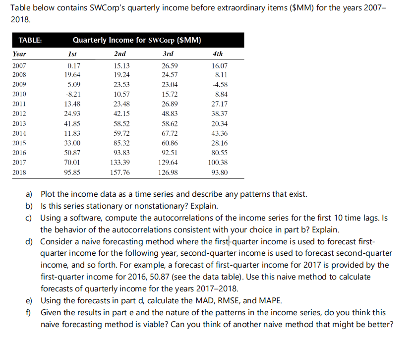
Table below contains SWCorp's quarterly income before extraordinary items ($MM) for the years 2007 2018. TABLE: Year 2007 2008 2009 2010 2011 2012 2013 2014 2015 2016 2017 2018 Quarterly Income for SWCorp ($MM) Ist 2nd 3rd 0.17 15.13 26.59 19.64 19.24 24.57 5.09 23.53 23.04 -8.21 10.57 15.72 13.48 23.48 26.89 24.93 42.15 48.83 41.85 58.52 58.62 11.83 59.72 67.72 33.00 85.32 60.86 50.87 93.83 92.51 70.01 133.39 129.64 95.85 157.76 126.98 4th 16.07 8.11 -4.58 8.84 27.17 38.37 20.34 43.36 28.16 80.55 100.38 93.80 a) Plot the income data as a time series and describe any patterns that exist. b) Is this series stationary or nonstationary? Explain. c) Using a software, compute the autocorrelations of the income series for the first 10 time lags. Is the behavior of the autocorrelations consistent with your choice in part b? Explain. d) Consider a naive forecasting method where the first quarter income is used to forecast first- quarter income for the following year, second-quarter income is used to forecast second-quarter income, and so forth. For example, a forecast of first-quarter income for 2017 is provided by the first-quarter income for 2016, 50.87 (see the data table). Use this naive method to calculate forecasts of quarterly income for the years 2017-2018. e) Using the forecasts in part de calculate the MAD, RMSE, and MAPE. f) Given the results in part e and the nature of the patterns in the income series, do you think this naive forecasting method is viable? Can you think of another naive method that might be better? Table below contains SWCorp's quarterly income before extraordinary items ($MM) for the years 2007 2018. TABLE: Year 2007 2008 2009 2010 2011 2012 2013 2014 2015 2016 2017 2018 Quarterly Income for SWCorp ($MM) Ist 2nd 3rd 0.17 15.13 26.59 19.64 19.24 24.57 5.09 23.53 23.04 -8.21 10.57 15.72 13.48 23.48 26.89 24.93 42.15 48.83 41.85 58.52 58.62 11.83 59.72 67.72 33.00 85.32 60.86 50.87 93.83 92.51 70.01 133.39 129.64 95.85 157.76 126.98 4th 16.07 8.11 -4.58 8.84 27.17 38.37 20.34 43.36 28.16 80.55 100.38 93.80 a) Plot the income data as a time series and describe any patterns that exist. b) Is this series stationary or nonstationary? Explain. c) Using a software, compute the autocorrelations of the income series for the first 10 time lags. Is the behavior of the autocorrelations consistent with your choice in part b? Explain. d) Consider a naive forecasting method where the first quarter income is used to forecast first- quarter income for the following year, second-quarter income is used to forecast second-quarter income, and so forth. For example, a forecast of first-quarter income for 2017 is provided by the first-quarter income for 2016, 50.87 (see the data table). Use this naive method to calculate forecasts of quarterly income for the years 2017-2018. e) Using the forecasts in part de calculate the MAD, RMSE, and MAPE. f) Given the results in part e and the nature of the patterns in the income series, do you think this naive forecasting method is viable? Can you think of another naive method that might be better