can you please solve this in formula form on excel with the formulas written out so i can see where the answers cam from please! can

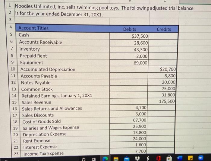
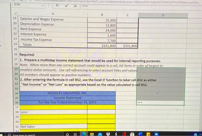
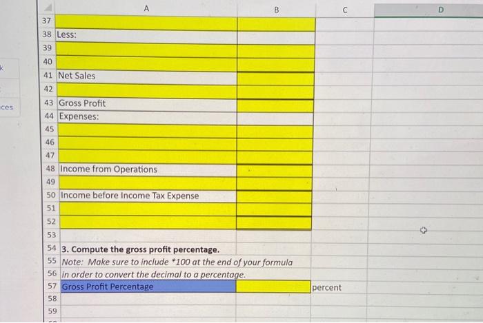
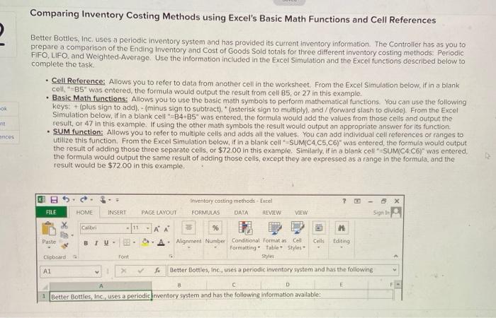
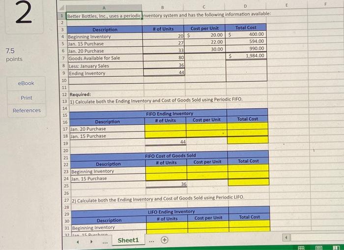
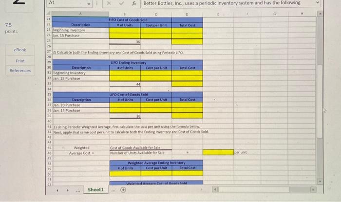
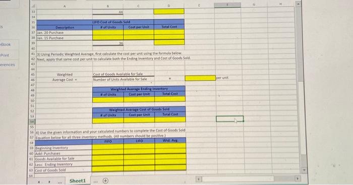
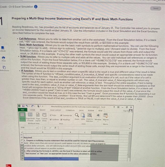
can you please solve it in formula form as well show the formula used so i can see where the solution is from

Credit - Ch 6 Excel Simulation Saved Preparing a Multi-Step Income Statement using Excel's IF and Basic Math Functions 1 cBook P Reading Readiness, Inc. has provided you its list of accounts and balances as of January 31. The Controller has asked you to prepare an Income Statement for the month ended January 31. Use the information included in the Excel Simulation and the Excel functions described below to complete the task. Coll Reference: Allows you to refer to data from another celt in the worksheet. From the Excel Simulation below, if in a blank cell"-35" was entered the formula would output the result from cell B5, or $37,500 in this example. Basic Math functions: Allows you to use the basic math symbols to perform mathematical functions You can use the following keys: + (plus sign to add) - (minus sign to subtract). * (asterisk sign to multiply), and / (forward slash to divide). From the Excel Simulation below.if in a blank cell =C11+C12" was entered the formula would add the values from those cells and output the result, or 28,800 in this example. If using the other math symbols the result would output an appropriate answer for its function SUM function: Allows you to refer to multiple cells and adds all the values You can add individual cell references or ranges to utilize this function. From the Excel Simulation below, if in a blank cell SUMC11, C12,C13)" was entered the formula would output the result of adding those three separate cells, or 103,800 in this example. Similarly, if in a blank cell =SUMC11:013)" was entered the formula would output the same result of adding those cells, except they are expressed as a range in the formula, and the result would be 103,800 in this example, IF function: Allows you to test a condition and return a specific value is the result is true and different value if the result is false. The syntax of the IF function is "IF(test_condition,value_il_true,value_Il_false)" and specific considerations need to be made when using this function. The test_condition argument is an evaluation of the status of a cell, such as if the value of a cellis greater than, less than or equal to another number or cell The value_l_true and value. Il faise arguments will return any specific result for each option, such as another cell reference, o value, or text. Throughout the entire equation, if text is being used in the test condition, value_true, or value_I false arguments then the text itself should be entered in quotations so that Excel will recognize the text as a string of text" instead of another function. From the Excel Simulation below, if in a blank cell IF(85-20000,"Cash is great", "Cash is bad") was entered the formula would output the result of the value it true since the test_condition would be result as true, or in this case the text "Cash is great". Excel processes the IF function by separating it out Into separate parts. First the tesLcondition-Excel thinks, find cell 85 and determine if the value is greater than 20000. Once Excel determines if the result of that test_condition is TRUE or FALSE, it will return the value. Il true or value I false. References FILE Marchandising operations and ther-step income statement Feel PALL LAYOUT FORMULAS DATA REVIEW VIEW 5 X Sign In Murer roma Goldlines Heading Home Page Break Page Custom Preview Layout Views Workbook Vw Zoom 100Zoom to Window Macro Selection Loom 036 A 25 26 Required: 27 1. Prepare a multistepincome statement that would be used for internal reporting purposes. 28. Note: When more than one correct account could appear in a cell list items in order ofgest to 29 mallest dolor amounts. Use cell referending to select accountities and value 10 All numbers should appear as pourive numbers 31 2. After entering the formula in cell B52, use the Excel IF function to label cell AS2 as ather 12 "Net Income" or "Net Loss as appropriate based on the value calculated in B52 1 19 NOODILSTUNUMITED, INC ME 4 Cash 6 1 Noodles Unlimited, Inc. sells swimming pool toys. The following adjusted trial balance 2 is for the year ended December 31, 20X1. 3 Account Titles Debits Credits 5 $37,500 Accounts Receivable 28,600 7 Inventory 43,300 8 Prepaid Rent 2,000 9 Equipment 69,000 10 Accumulated Depreciation $20,700 11 Accounts Payable 8,800 12 Notes Payable 20,000 13 Common Stock 75,000 14 Retained Earnings, January 1, 20X1 31,800 Sales Revenue 175,500 16 Sales Returns and Allowances 4,700 17 Sales Discounts 6,000 18 Cost of Goods Sold 67,700 19 Salaries and Wages Expense 25,900 20 Depreciation Expense 13,800 21 Rent Expense 24,000 22 Interest Expense 1,600 7,700 Income Tax Expense 15 23 d - C D36 ezte meducation.com/ext/map/index.html?con con&external browser0&launchurt-https%253A%252F%252Flearn.csuchico Jx A 5 B C D 19 Salaries and Wages Expense 25,900 20 Depreciation Expense 13,800 21 Rent Expense 24,000 22 Interest Expense 1,600 23 Income Tax Expense 7,700 24 Totals $331,800 $331,800 25 26 Required: 27 1. Prepare a multistep income statement that would be used for internal reporting purposes. 28. Note: When more than one correct account could appear in a cell, list items in order of largest to 29 smallest dollar amounts. Use cell referencing to select account titles and values 30 All numbers should appear as positive numbers. 31 2. After entering the formula in cell B52, use the Excel IF function to label cell A52 as either 32 "Net Income" or "Net Loss" as appropriate based on the value calculated in dell B52. NOODLES UNLIMITED, INC. 35 Income Statement 36 For the Year Ended December 31, 20X1 37 38 Less: 39 40 41 Net Sales 33 34 +++ Tractatutch O A B C D 37 38 Less: 39 k ces 40 41 Net Sales 42 43 Gross Profit 44 Expenses: 45 46 47 48 Income from Operations 49 50 Income before Income Tax Expense 51 52 53 54 3. Compute the gross profit percentage. 55 Note: Make sure to include *100 at the end of your formula 56 In order to convert the decimal to a percentage. 57 Gross Profit Percentage percent 58 59 Comparing Inventory Costing Methods using Excel's Basic Math Functions and Cell References Better Bottles, Inc. uses a periodic inventory system and has provided its current inventory information. The Controller has as you to prepare a comparison of the Ending Inventory and cost of Goods Sold totals for three different inventory costing methods Periodic FIFO, LIFO and Weighted-Average. Use the information included in the Excel Simulation and the Excel functions described below to complete the task Cell Reference: Allows you to refer to data from another cell in the worksheet. From the Excel Simulation below, if in a blank cell, B5" was entered, the formula would output the result from cell B5, or 27 in this example. Basic Math functions: Allows you to use the basic math symbols to perform mathematical functions. You can use the following keys (plus sign to add). - (minus sign to subtract). (asterisk sign to multiply), and / (forward slash to divide). From the Excel Simulation below, if in a blank cellB4-B5" was entered the formula would add the values from those cells and output the result, or 47 in this example. If using the other math symbols the result would output an appropriate answer for its function SUM function: Allows you to refer to multiple cells and adds all the values. You can add individual cell references or ranges to utilize this function. From the Excel Simulation below, if in a blank cell SUMC4,C5,C6)" was entered the formula would output the result of adding those three separate cells, or $72.00 in this example. Similarly, if in a blank cell SUMC4C6)" was entered, the formula would output the same result of adding those cells, except they are expressed as a range in the formula and the result would be $72.00 in this example ances KI Inventory costing methods - Excel FORMULAS DATA SEVIEW 3 x son FILE HOME INSERT PAGE LAYOUT VIEW X Con H Editing Paste -AA % AA. Alignment Number Conditional Formatan Cel Formatting Table Styles Styles Cells BTU- Clipboard Font AL Better Bottles, Inc., uses a periodic inventory system and has the following E A D 1 Better Bottles, Inc., uses a periodic inventory system and has the following information available: E 2 7.5 points eBook Print References B D 1 Better Bottles, Inc. uses a periodic nventory system and has the following information available: 2 3 Description # of Units Cost per Unit Total Cost 4 Beginning Inventory 20 S 20.00 S 400.00 5 Jan, 15 Purchase 27 22.00 594.00 6 Jan. 20 Purchase 33 30.00 990.00 7 Goods Available for Sale 80 $ 1984.00 8 Less: January Sales 36 9 Ending Inventory 44 10 11 12 Required: 13 1) Calculate both the Ending Inventory and Cost of Goods Sold using Periodic FIFO. 14 15 FIFO Ending Inventory 16 Description # of Units Cost per Unit Total Cost 17 Jan. 20 Purchase 18 Jan. 15 Purchase 19 44 20 21 FIFO Cost of Goods Sold 22 Description # of Units Cost per Unit Total Cost 23 Beginning Inventory 24 Jan. 15 Purchase 25 36 26 27 2) Calculate both the Ending Inventory and Cost of Goods Sold using Periodic LiFO 28 29 LIFO Ending Inventory 30 Description # of Units Cost per Unit Total Cost 31 Beginning Inventory 32 i 16 Ducha Sheet1 HHH 2 A1 Better Bottles, Inc., uses a periodic inventory system and has the following 75 points eBook Print References c. 21 FIFO Cost of Goods Sold 22 Description of Units Cort per Unit Total Con 23 Beginning inventory 24 Jan. 15 Purchase 25 35 26 272) Calculate both the Ending inventory and cost of Goods Sold using Periodic LIFO 28 29 UFO Ending Inventory 30 Description of Units Cost per Unit Total Cost 31 Beginning inventory 32 lan 15 Purchase 33 14 35 LIFO Cost of Goods Sold 36 Description of Units Cost per unit Total Cont 37 Jan 20 Purchase 38 a 15 Purchase 39 40 413) Using Periodic Weighted Average first calculate the cost per units the form below 42 Next, apply the same cost per unit to calculate both the Ending Inventory and cost of Goods Sold 43 44 45 Weighted Costo da Alable for Sale 46 Average cost Number of Units Available for Sale 47 Weighted Average Endir inventory of Units Cost per Unit Total Cost 50 SI 52 Welated Averare code Sheet1 Der 993 - D E 44 35 es LIFDC of God Description of Us Con per Unit Total Cost IR 20 Purchase 10. Purchase 19 40 453) Using Periodic Welighted Average first calculate the cost per unit using the formula below 42 Next, apply that same cost per unit to calculate both the Ending Invertory and Cost of Goods Sold -Book Print rences 43 Weighted Avenge Cost Chiot Godalable for sale Number of Units Available for Sale per unit 47 41 40 SD Weighted Average Inding Inventory of Unite Cost per Unit Total Cost 53 Weighted Average Cost podsed Con per Unit Total Cost 55 564 Use the given information and your calculated numbers to complete the cost of Goods Sold 37 ton below for all the inventoryhod Allumtur thould be 18 FO fo Wid. AVE Berwentory 60 Ade Purchases 01 Goods Avatable for Sale 2 less Endir inventary A cost of Good Sold Sheet1 Credit - Ch 6 Excel Simulation Saved Preparing a Multi-Step Income Statement using Excel's IF and Basic Math Functions 1 cBook P Reading Readiness, Inc. has provided you its list of accounts and balances as of January 31. The Controller has asked you to prepare an Income Statement for the month ended January 31. Use the information included in the Excel Simulation and the Excel functions described below to complete the task. Coll Reference: Allows you to refer to data from another celt in the worksheet. From the Excel Simulation below, if in a blank cell"-35" was entered the formula would output the result from cell B5, or $37,500 in this example. Basic Math functions: Allows you to use the basic math symbols to perform mathematical functions You can use the following keys: + (plus sign to add) - (minus sign to subtract). * (asterisk sign to multiply), and / (forward slash to divide). From the Excel Simulation below.if in a blank cell =C11+C12" was entered the formula would add the values from those cells and output the result, or 28,800 in this example. If using the other math symbols the result would output an appropriate answer for its function SUM function: Allows you to refer to multiple cells and adds all the values You can add individual cell references or ranges to utilize this function. From the Excel Simulation below, if in a blank cell SUMC11, C12,C13)" was entered the formula would output the result of adding those three separate cells, or 103,800 in this example. Similarly, if in a blank cell =SUMC11:013)" was entered the formula would output the same result of adding those cells, except they are expressed as a range in the formula, and the result would be 103,800 in this example, IF function: Allows you to test a condition and return a specific value is the result is true and different value if the result is false. The syntax of the IF function is "IF(test_condition,value_il_true,value_Il_false)" and specific considerations need to be made when using this function. The test_condition argument is an evaluation of the status of a cell, such as if the value of a cellis greater than, less than or equal to another number or cell The value_l_true and value. Il faise arguments will return any specific result for each option, such as another cell reference, o value, or text. Throughout the entire equation, if text is being used in the test condition, value_true, or value_I false arguments then the text itself should be entered in quotations so that Excel will recognize the text as a string of text" instead of another function. From the Excel Simulation below, if in a blank cell IF(85-20000,"Cash is great", "Cash is bad") was entered the formula would output the result of the value it true since the test_condition would be result as true, or in this case the text "Cash is great". Excel processes the IF function by separating it out Into separate parts. First the tesLcondition-Excel thinks, find cell 85 and determine if the value is greater than 20000. Once Excel determines if the result of that test_condition is TRUE or FALSE, it will return the value. Il true or value I false. References FILE Marchandising operations and ther-step income statement Feel PALL LAYOUT FORMULAS DATA REVIEW VIEW 5 X Sign In Murer roma Goldlines Heading Home Page Break Page Custom Preview Layout Views Workbook Vw Zoom 100Zoom to Window Macro Selection Loom 036 A 25 26 Required: 27 1. Prepare a multistepincome statement that would be used for internal reporting purposes. 28. Note: When more than one correct account could appear in a cell list items in order ofgest to 29 mallest dolor amounts. Use cell referending to select accountities and value 10 All numbers should appear as pourive numbers 31 2. After entering the formula in cell B52, use the Excel IF function to label cell AS2 as ather 12 "Net Income" or "Net Loss as appropriate based on the value calculated in B52 1 19 NOODILSTUNUMITED, INC ME 4 Cash 6 1 Noodles Unlimited, Inc. sells swimming pool toys. The following adjusted trial balance 2 is for the year ended December 31, 20X1. 3 Account Titles Debits Credits 5 $37,500 Accounts Receivable 28,600 7 Inventory 43,300 8 Prepaid Rent 2,000 9 Equipment 69,000 10 Accumulated Depreciation $20,700 11 Accounts Payable 8,800 12 Notes Payable 20,000 13 Common Stock 75,000 14 Retained Earnings, January 1, 20X1 31,800 Sales Revenue 175,500 16 Sales Returns and Allowances 4,700 17 Sales Discounts 6,000 18 Cost of Goods Sold 67,700 19 Salaries and Wages Expense 25,900 20 Depreciation Expense 13,800 21 Rent Expense 24,000 22 Interest Expense 1,600 7,700 Income Tax Expense 15 23 d - C D36 ezte meducation.com/ext/map/index.html?con con&external browser0&launchurt-https%253A%252F%252Flearn.csuchico Jx A 5 B C D 19 Salaries and Wages Expense 25,900 20 Depreciation Expense 13,800 21 Rent Expense 24,000 22 Interest Expense 1,600 23 Income Tax Expense 7,700 24 Totals $331,800 $331,800 25 26 Required: 27 1. Prepare a multistep income statement that would be used for internal reporting purposes. 28. Note: When more than one correct account could appear in a cell, list items in order of largest to 29 smallest dollar amounts. Use cell referencing to select account titles and values 30 All numbers should appear as positive numbers. 31 2. After entering the formula in cell B52, use the Excel IF function to label cell A52 as either 32 "Net Income" or "Net Loss" as appropriate based on the value calculated in dell B52. NOODLES UNLIMITED, INC. 35 Income Statement 36 For the Year Ended December 31, 20X1 37 38 Less: 39 40 41 Net Sales 33 34 +++ Tractatutch O A B C D 37 38 Less: 39 k ces 40 41 Net Sales 42 43 Gross Profit 44 Expenses: 45 46 47 48 Income from Operations 49 50 Income before Income Tax Expense 51 52 53 54 3. Compute the gross profit percentage. 55 Note: Make sure to include *100 at the end of your formula 56 In order to convert the decimal to a percentage. 57 Gross Profit Percentage percent 58 59 Comparing Inventory Costing Methods using Excel's Basic Math Functions and Cell References Better Bottles, Inc. uses a periodic inventory system and has provided its current inventory information. The Controller has as you to prepare a comparison of the Ending Inventory and cost of Goods Sold totals for three different inventory costing methods Periodic FIFO, LIFO and Weighted-Average. Use the information included in the Excel Simulation and the Excel functions described below to complete the task Cell Reference: Allows you to refer to data from another cell in the worksheet. From the Excel Simulation below, if in a blank cell, B5" was entered, the formula would output the result from cell B5, or 27 in this example. Basic Math functions: Allows you to use the basic math symbols to perform mathematical functions. You can use the following keys (plus sign to add). - (minus sign to subtract). (asterisk sign to multiply), and / (forward slash to divide). From the Excel Simulation below, if in a blank cellB4-B5" was entered the formula would add the values from those cells and output the result, or 47 in this example. If using the other math symbols the result would output an appropriate answer for its function SUM function: Allows you to refer to multiple cells and adds all the values. You can add individual cell references or ranges to utilize this function. From the Excel Simulation below, if in a blank cell SUMC4,C5,C6)" was entered the formula would output the result of adding those three separate cells, or $72.00 in this example. Similarly, if in a blank cell SUMC4C6)" was entered, the formula would output the same result of adding those cells, except they are expressed as a range in the formula and the result would be $72.00 in this example ances KI Inventory costing methods - Excel FORMULAS DATA SEVIEW 3 x son FILE HOME INSERT PAGE LAYOUT VIEW X Con H Editing Paste -AA % AA. Alignment Number Conditional Formatan Cel Formatting Table Styles Styles Cells BTU- Clipboard Font AL Better Bottles, Inc., uses a periodic inventory system and has the following E A D 1 Better Bottles, Inc., uses a periodic inventory system and has the following information available: E 2 7.5 points eBook Print References B D 1 Better Bottles, Inc. uses a periodic nventory system and has the following information available: 2 3 Description # of Units Cost per Unit Total Cost 4 Beginning Inventory 20 S 20.00 S 400.00 5 Jan, 15 Purchase 27 22.00 594.00 6 Jan. 20 Purchase 33 30.00 990.00 7 Goods Available for Sale 80 $ 1984.00 8 Less: January Sales 36 9 Ending Inventory 44 10 11 12 Required: 13 1) Calculate both the Ending Inventory and Cost of Goods Sold using Periodic FIFO. 14 15 FIFO Ending Inventory 16 Description # of Units Cost per Unit Total Cost 17 Jan. 20 Purchase 18 Jan. 15 Purchase 19 44 20 21 FIFO Cost of Goods Sold 22 Description # of Units Cost per Unit Total Cost 23 Beginning Inventory 24 Jan. 15 Purchase 25 36 26 27 2) Calculate both the Ending Inventory and Cost of Goods Sold using Periodic LiFO 28 29 LIFO Ending Inventory 30 Description # of Units Cost per Unit Total Cost 31 Beginning Inventory 32 i 16 Ducha Sheet1 HHH 2 A1 Better Bottles, Inc., uses a periodic inventory system and has the following 75 points eBook Print References c. 21 FIFO Cost of Goods Sold 22 Description of Units Cort per Unit Total Con 23 Beginning inventory 24 Jan. 15 Purchase 25 35 26 272) Calculate both the Ending inventory and cost of Goods Sold using Periodic LIFO 28 29 UFO Ending Inventory 30 Description of Units Cost per Unit Total Cost 31 Beginning inventory 32 lan 15 Purchase 33 14 35 LIFO Cost of Goods Sold 36 Description of Units Cost per unit Total Cont 37 Jan 20 Purchase 38 a 15 Purchase 39 40 413) Using Periodic Weighted Average first calculate the cost per units the form below 42 Next, apply the same cost per unit to calculate both the Ending Inventory and cost of Goods Sold 43 44 45 Weighted Costo da Alable for Sale 46 Average cost Number of Units Available for Sale 47 Weighted Average Endir inventory of Units Cost per Unit Total Cost 50 SI 52 Welated Averare code Sheet1 Der 993 - D E 44 35 es LIFDC of God Description of Us Con per Unit Total Cost IR 20 Purchase 10. Purchase 19 40 453) Using Periodic Welighted Average first calculate the cost per unit using the formula below 42 Next, apply that same cost per unit to calculate both the Ending Invertory and Cost of Goods Sold -Book Print rences 43 Weighted Avenge Cost Chiot Godalable for sale Number of Units Available for Sale per unit 47 41 40 SD Weighted Average Inding Inventory of Unite Cost per Unit Total Cost 53 Weighted Average Cost podsed Con per Unit Total Cost 55 564 Use the given information and your calculated numbers to complete the cost of Goods Sold 37 ton below for all the inventoryhod Allumtur thould be 18 FO fo Wid. AVE Berwentory 60 Ade Purchases 01 Goods Avatable for Sale 2 less Endir inventary A cost of Good Sold Sheet1