Case questions:

1. Compute expected return and standard deviation of annual return for each alternative separately.

2. Compute covariance of annual returns between the Alaska and Houston offices, and between the California and Houston offices.

3. Compute the expected return and standard deviation for each of the two combinations.

4. Prepare pro forma statements for each new office combined with the Houston office, using each of the four possible conditions.

5. What would you recommend to Cotner? Why?

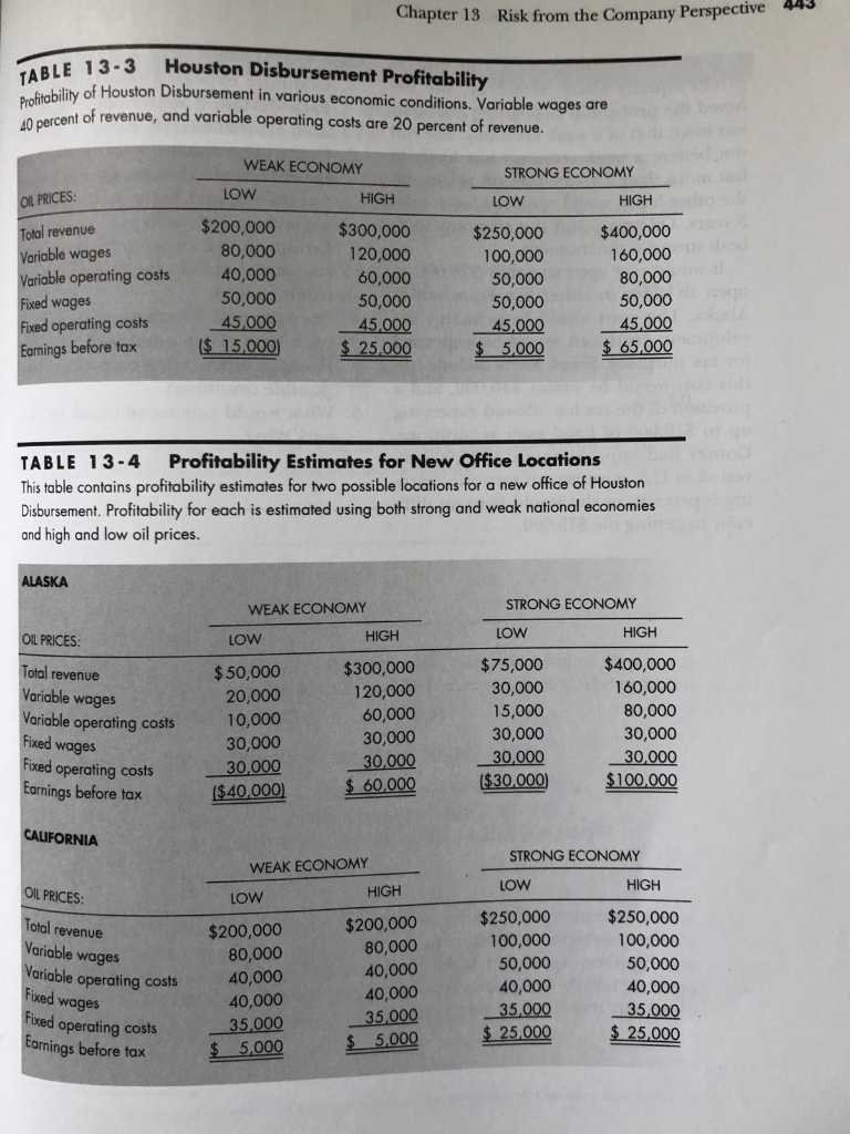
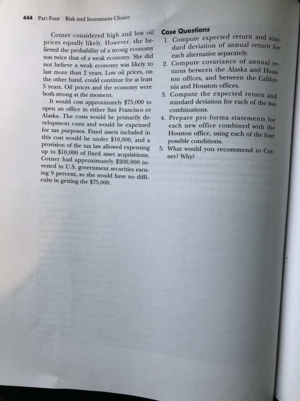
442 Part Four Risk and Investment Choice buy an interest in calize that she CASE PROBLEM Houston Disbursement y Cotner went to work for a title com- that he could eventually buy an inter y after graduating from college. The Houston Disbursement. department she worked in provided dis- Cotner soon came to realize that bursement advice to banks with regard to had gained little from diversification oil/gas-related loans. When a bank drop in oil prices caused the entire Houe granted a construction loan, the money ton economy to turn down, even when the was paid out according to progress made. national economy was strong. Based on Someone had to monitor the project and her experiences, Cotner prepared an eerd authorize disbursement of cash under the mate of revenue and profits for Houston loan agreement. While most banks moni- Disbursement for both a strong and a weak tor progress themselves, a few rely on out- economy, and for both high and low oil side firms to do the monitoring, and this is prices. Her estimates are summarized in what Cotner's department did. Table 13-3. While the analysis focuses on Cotner spent nearly a decade learning earnings before tax, this is approximately the business and working her way up to as- the same as cash flow because capital in- sistant manager of the department. Then vestments were limited to office furniture, a recession caused a decline in profits for and net working capital was negligible. Net the title company. The title company de- working capital was kept negligible by the cided to get out of oil/gas disbursement, practice of collecting retainer fees from and the department manager decided to banks at the start of a construction project. retire. Cotner's salary, based on her estimate of Cotner thought that there was still what she could get if she were working for enough business to make a decent living another company, is included in the cost for herself if she did not have to bear the figures. The business was organized as a overhead cost of the title company. As she Subchapter S corporation and Cotner was informed the lenders of the title com- in a 28 percent tax bracket. pany's decision, she also informed them To diversify, Cotner decided to open a that she would be opening her own office. second office. She would go to the new lo- She had developed an excellent personal cation and promote Ross to manager of the reputation, and several major lenders indi- Houston office. Two possibilities that would cated a willingness to continue doing busi- take advantage of her current contacts were ness with her. Thus, Houston Disburse- a commercial construction disbursement ment was born. office in San Francisco and an oil business As the recession ended, Cotner's busi- disbursement office in Alaska. Cotner was ness picked up substantially, but she quite willing to move to either area. began to worry about the vagaries of the Cotner's estimates of profitability ap oil business. She decided to diversify into pear in Table 13-4. The costs include a fall general commercial construction in the wage for Cotner; there would be no signil Houston area. She hired Brent Ross, a ed brent Koss, a icant wage savings at the Houston office icant wage sav young loan officer in the commercial con- because a struction field, with the understanding be needed. Chapter 13 Risk from the Company Perspective 443 AL 13-3 Houston Disbursement Profitability Wbility of Houston Disbursement in various economic conditions. Variable wages are cent of revenue, and variable operating costs are 20 percent of revenue. Profitability of Ho OIL PRICES: O Total revenue Variable wages Variable operating costs Fixed wages Fixed operating costs Earnings before tax WEAK ECONOMY LOW HIGH $200,000 $300,000 80,000 120,000 40,000 60,000 50,000 50,000 45,000 45,000 ($ 15,000 $ 25,000 STRONG ECONOMY LOW HIGH $250,000 $400,000 100,000 160,000 50,000 80,000 50,000 50,000 45,000 45,000 $ 5,000 $ 65,000 TABLE 13-4 Profitability Estimates for New Office Locations This table contains profitability estimates for two possible locations for a new office of Houston Disbursement. Profitability for each is estimated using both strong and weak national economies and high and low oil prices. ALASKA OIL PRICES: Total revenue Variable wages Variable operating costs Fixed wages Fixed operating costs Earnings before tax WEAK ECONOMY LOW HIGH $50,000 $300,000 20,000 120,000 10,000 60,000 30,000 30,000 30,000 30,000 ($40,000) $ 60,000 STRONG ECONOMY LOW HIGH $75,000 $400,000 30,000 160,000 15,000 80,000 30,000 30,000 30,000 30,000 ($30,000) $100,000 CALIFORNIA OIL PRICES: Total revenue Variable wages WEAK ECONOMY LOW HIGH $200,000 $200,000 80,000 80,000 40,000 40,000 40,000 40,000 35,000 35,000 $ 5.000 $ 5,000 STRONG ECONOMY LOW HIGH $250,000 $250,000 100,000 100,000 50,000 50,000 40,000 40,000 35,000 35,000 $ 25,000 $ 25,000 Variable operating costs Fixed wages Fixed operating costs Earnings before tax 444 Part Four Risk and Investment Choice Cotner considered high and low oil Case Questions 1. Compute expected return and st prices equally likely. However, she be- dard deviation of annual return moved the probability of a strong economy was twice that of a weak economy. She did each alternative separately. MOL believe a weak economy was likely to 2. Compute covariance of annual last more than 2 years. Low oil prices, on turns between the Alaska and Hone the other hand, could continue for at least ton offices, and between the Califor. 5 years. Oil prices and the economy were nia and Houston offices. both strong at the moment. 3. Compute the expected return and It would cost approximately $75,000 to standard deviation for each of the two open an office in either San Francisco or combinations. Alaska. The costs would be primarily de- 4. Prepare pro forma statements for velopment costs and would be expensed each new office combined with the for tax purposes. Fixed assets included in Houston office, using each of the four this cost would be under $10,000, and a possible conditions. provision of the tax law allowed expensing 5. What would you recommend to Cot- up to $10,000 of fixed asset acquisitions. Cotner had approximately $200,000 in- ner? Why? vested in U.S. government securities earn- ing 9 percent, so she would have no diffi- culty in getting the $75,000. 442 Part Four Risk and Investment Choice buy an interest in calize that she CASE PROBLEM Houston Disbursement y Cotner went to work for a title com- that he could eventually buy an inter y after graduating from college. The Houston Disbursement. department she worked in provided dis- Cotner soon came to realize that bursement advice to banks with regard to had gained little from diversification oil/gas-related loans. When a bank drop in oil prices caused the entire Houe granted a construction loan, the money ton economy to turn down, even when the was paid out according to progress made. national economy was strong. Based on Someone had to monitor the project and her experiences, Cotner prepared an eerd authorize disbursement of cash under the mate of revenue and profits for Houston loan agreement. While most banks moni- Disbursement for both a strong and a weak tor progress themselves, a few rely on out- economy, and for both high and low oil side firms to do the monitoring, and this is prices. Her estimates are summarized in what Cotner's department did. Table 13-3. While the analysis focuses on Cotner spent nearly a decade learning earnings before tax, this is approximately the business and working her way up to as- the same as cash flow because capital in- sistant manager of the department. Then vestments were limited to office furniture, a recession caused a decline in profits for and net working capital was negligible. Net the title company. The title company de- working capital was kept negligible by the cided to get out of oil/gas disbursement, practice of collecting retainer fees from and the department manager decided to banks at the start of a construction project. retire. Cotner's salary, based on her estimate of Cotner thought that there was still what she could get if she were working for enough business to make a decent living another company, is included in the cost for herself if she did not have to bear the figures. The business was organized as a overhead cost of the title company. As she Subchapter S corporation and Cotner was informed the lenders of the title com- in a 28 percent tax bracket. pany's decision, she also informed them To diversify, Cotner decided to open a that she would be opening her own office. second office. She would go to the new lo- She had developed an excellent personal cation and promote Ross to manager of the reputation, and several major lenders indi- Houston office. Two possibilities that would cated a willingness to continue doing busi- take advantage of her current contacts were ness with her. Thus, Houston Disburse- a commercial construction disbursement ment was born. office in San Francisco and an oil business As the recession ended, Cotner's busi- disbursement office in Alaska. Cotner was ness picked up substantially, but she quite willing to move to either area. began to worry about the vagaries of the Cotner's estimates of profitability ap oil business. She decided to diversify into pear in Table 13-4. The costs include a fall general commercial construction in the wage for Cotner; there would be no signil Houston area. She hired Brent Ross, a ed brent Koss, a icant wage savings at the Houston office icant wage sav young loan officer in the commercial con- because a struction field, with the understanding be needed. Chapter 13 Risk from the Company Perspective 443 AL 13-3 Houston Disbursement Profitability Wbility of Houston Disbursement in various economic conditions. Variable wages are cent of revenue, and variable operating costs are 20 percent of revenue. Profitability of Ho OIL PRICES: O Total revenue Variable wages Variable operating costs Fixed wages Fixed operating costs Earnings before tax WEAK ECONOMY LOW HIGH $200,000 $300,000 80,000 120,000 40,000 60,000 50,000 50,000 45,000 45,000 ($ 15,000 $ 25,000 STRONG ECONOMY LOW HIGH $250,000 $400,000 100,000 160,000 50,000 80,000 50,000 50,000 45,000 45,000 $ 5,000 $ 65,000 TABLE 13-4 Profitability Estimates for New Office Locations This table contains profitability estimates for two possible locations for a new office of Houston Disbursement. Profitability for each is estimated using both strong and weak national economies and high and low oil prices. ALASKA OIL PRICES: Total revenue Variable wages Variable operating costs Fixed wages Fixed operating costs Earnings before tax WEAK ECONOMY LOW HIGH $50,000 $300,000 20,000 120,000 10,000 60,000 30,000 30,000 30,000 30,000 ($40,000) $ 60,000 STRONG ECONOMY LOW HIGH $75,000 $400,000 30,000 160,000 15,000 80,000 30,000 30,000 30,000 30,000 ($30,000) $100,000 CALIFORNIA OIL PRICES: Total revenue Variable wages WEAK ECONOMY LOW HIGH $200,000 $200,000 80,000 80,000 40,000 40,000 40,000 40,000 35,000 35,000 $ 5.000 $ 5,000 STRONG ECONOMY LOW HIGH $250,000 $250,000 100,000 100,000 50,000 50,000 40,000 40,000 35,000 35,000 $ 25,000 $ 25,000 Variable operating costs Fixed wages Fixed operating costs Earnings before tax 444 Part Four Risk and Investment Choice Cotner considered high and low oil Case Questions 1. Compute expected return and st prices equally likely. However, she be- dard deviation of annual return moved the probability of a strong economy was twice that of a weak economy. She did each alternative separately. MOL believe a weak economy was likely to 2. Compute covariance of annual last more than 2 years. Low oil prices, on turns between the Alaska and Hone the other hand, could continue for at least ton offices, and between the Califor. 5 years. Oil prices and the economy were nia and Houston offices. both strong at the moment. 3. Compute the expected return and It would cost approximately $75,000 to standard deviation for each of the two open an office in either San Francisco or combinations. Alaska. The costs would be primarily de- 4. Prepare pro forma statements for velopment costs and would be expensed each new office combined with the for tax purposes. Fixed assets included in Houston office, using each of the four this cost would be under $10,000, and a possible conditions. provision of the tax law allowed expensing 5. What would you recommend to Cot- up to $10,000 of fixed asset acquisitions. Cotner had approximately $200,000 in- ner? Why? vested in U.S. government securities earn- ing 9 percent, so she would have no diffi- culty in getting the $75,000