Casey Hardware Stores Scenario Casey Hardware Stores is considering a location for a new store. Examining the profitability of its 20 stores for last year is a step that will help them make this decision. Leadership has decided to use linear regression analysis methods to determine if a linear correlation exists between the profits of its stores and the sales volume of its stores. It is hoped that this information and additional analyses will inform a decision on where to locate a future store. Part A: The management team initially wants to use Excel Linear Regression Analysis to take the data for the 20 stores that is in Table 1 to develop a best fit linear equation of the form: Y = a + b X1 where Y is the profit and X1 is the sales level. They are interested in seeing if there is a relationship between the profit and the sales levels of their 20 stores. Table 1 is a summary of Casey Hardware stores' performance, profits versus sales.

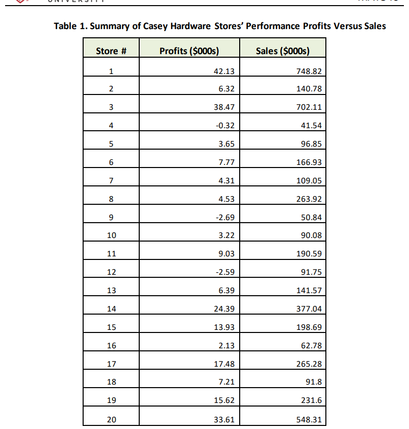
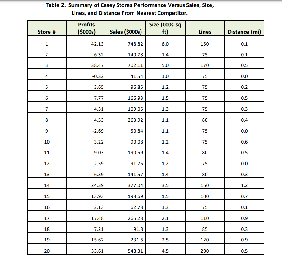
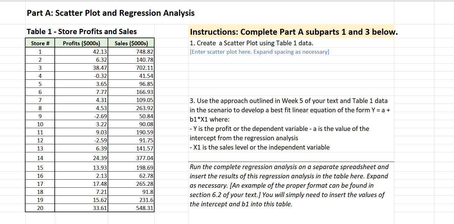
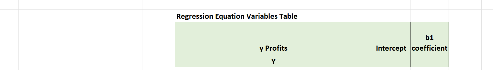
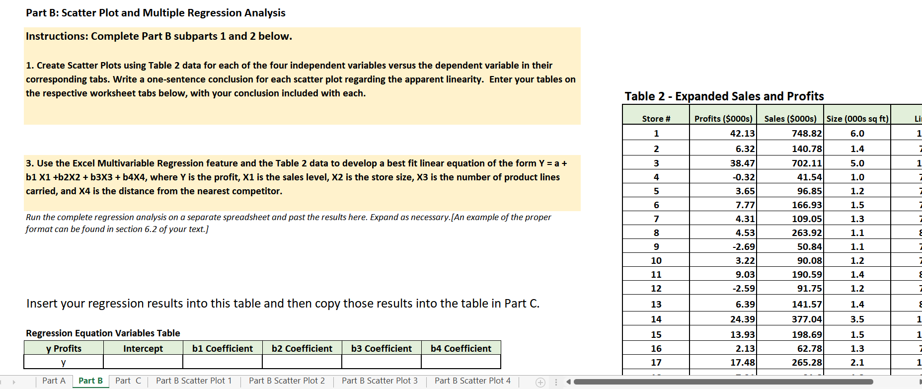
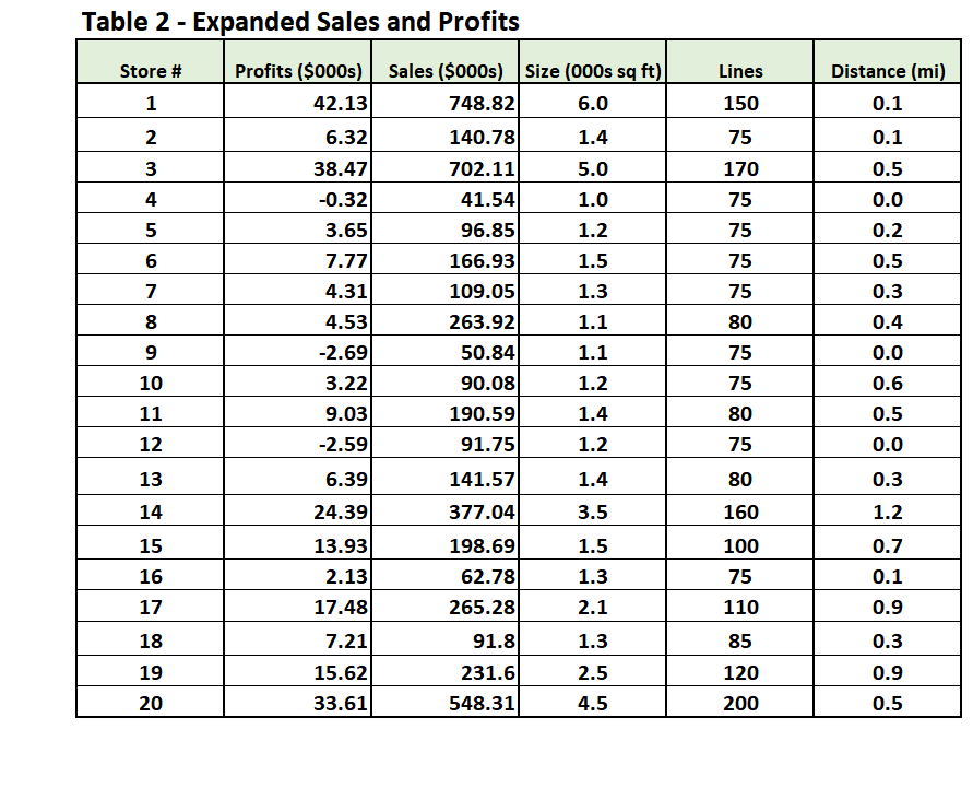
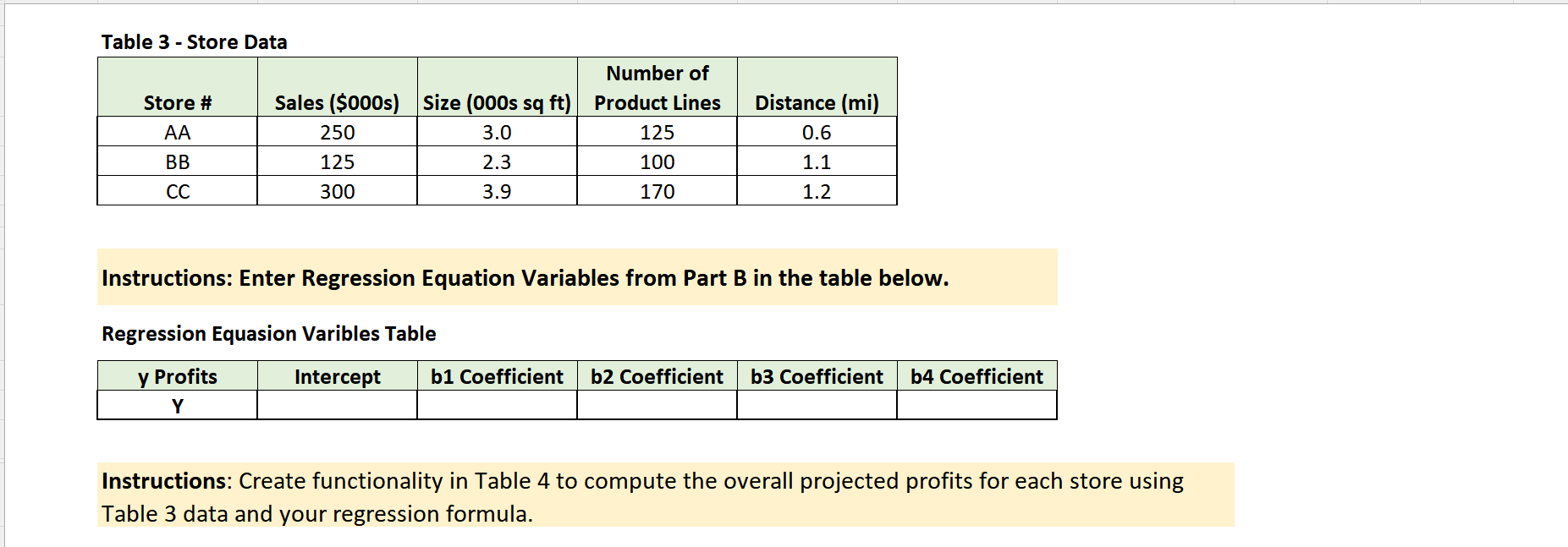
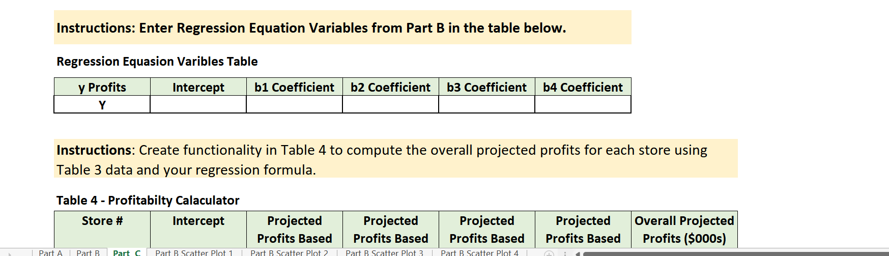
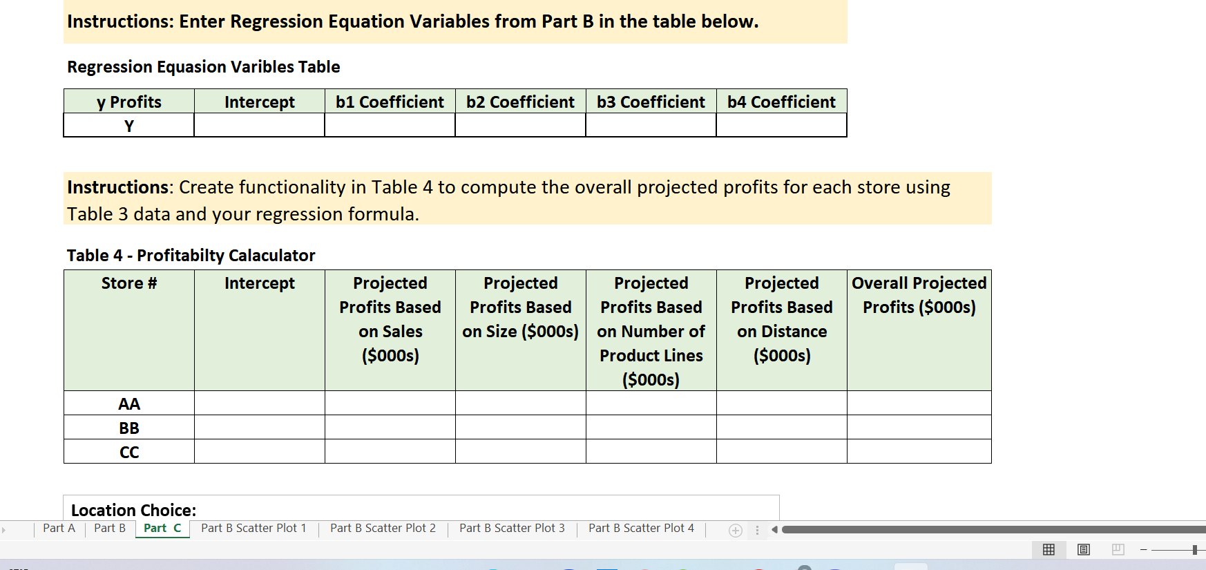
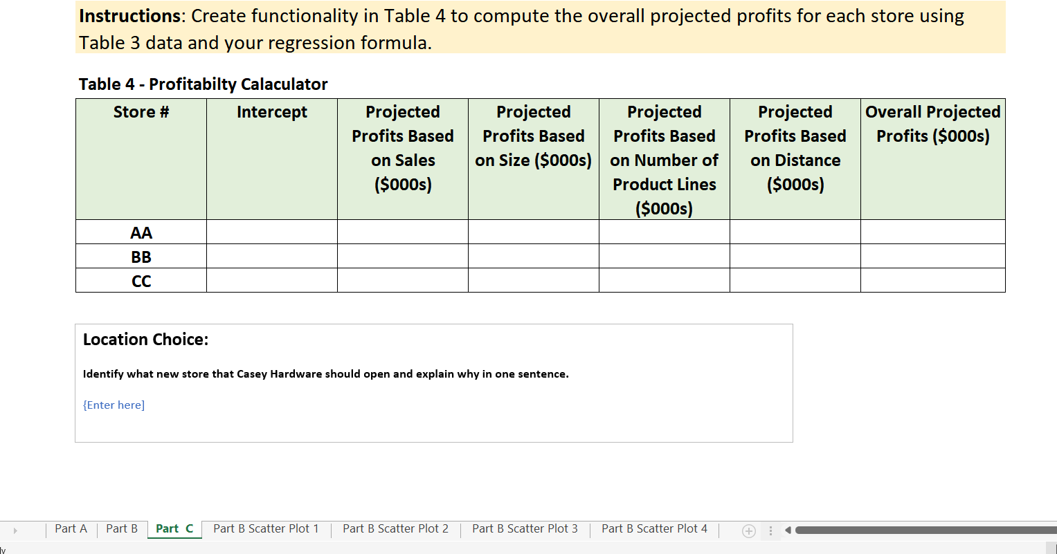
Table 1. Summary of Casey Hardware Stores' Performance Profits Versus Sales Store # Profits ($000s) Sales ($000s) 42.13 748.82 140.78 IN 5.32 3 38.47 702.11 -0.32 41.54 3.65 96.85 7.77 166.93 4.31 109.05 8 4.53 263.92 -2.69 50.84 10 3.22 90.08 11 9.03 190.59 12 -2.59 91.75 13 6.39 141.57 14 24.39 377.04 15 13.93 198.69 16 2.13 62.78 17 17.48 265.28 18 7.21 91.8 19 15.62 231.6 20 33.61 548.31Table 2. Summary of Casey Stores Performance Versus Sales, Size, Lines, and Distance From Nearest Competitor. Profits Size (000s sq Store # ($000s) Sales ($000s) ft) Lines Distance (mi) 42.13 748.82 6.0 150 0.1 IN 6.32 140.78 1.4 75 0.1 w 38.47 702.11 5.0 170 0.5 -0.32 41.54 1.0 75 0.0 3.65 96.85 1.2 75 0.2 7.77 166.93 1.5 75 0.5 4.31 109.05 1.3 75 0.3 4.53 263.92 1.1 80 0.4 -2.69 50.84 1.1 75 0.0 10 3.22 90.08 1.2 75 0.6 11 9.03 190.59 1.4 80 0.5 12 -2.59 91.75 1.2 75 0.0 13 5.39 141.57 1.4 80 0.3 14 24.39 377.04 3.5 160 1.2 15 13.93 198.69 1.5 100 0.7 16 2.13 62.78 1.3 75 0.1 17 17.48 265.28 2.1 0.9 18 7.21 91.8 1.3 85 0.3 19 15.62 231.6 2.5 120 0.9 20 33.61 548.31 4.5 200 0.5Part A: Scatter Plot and Regression Analysis Table 1 - Store Profits and Sales Instructions: Complete Part A subparts 1 and 3 below. Store # Profits ($000s) Sales ($000s) 1. Create a Scatter Plot using Table 1 data. 42.13 748.82 [Enter scatter plot here. Expand spacing as necessary] IN 6.32 140.78 W 38.47 702.11 -0.32 41.54 5 3.65 96.85 7.77 166.93 4.31 109.05 3. Use the approach outlined in Week 5 of your text and Table 1 data 4.53 263.92 in the scenario to develop a best fit linear equation of the form Y = a + 9 -2.69 50.84 b1*X1 where: 10 3.22 90.08 11 9.03 190.59 - Y is the profit or the dependent variable - a is the value of the 12 -2.59 91.75 intercept from the regression analysis 13 6.39 141.57 - X1 is the sales level or the independent variable 14 24.39 377.04 15 13.93 198.69 Run the complete regression analysis on a separate spreadsheet and 16 2.13 62.78 insert the results of this regression analysis in the table here. Expand 17 17.48 265.28 as necessary. [An example of the proper format can be found in 18 7.21 91.8 section 6.2 of your text.] You will simply need to insert the values of 19 15.62 231.6 20 33.61 548.31 the intercept and b1 into this table.Regression Equation Variables Table b1 y Profits Intercept coefficient YPart B: Scatter Plot and Multiple Regression Analysis Instructions: Complete Part B subparts 1 and 2 below. 1. Create Scatter Plots using Table 2 data for each of the four independent variables versus the dependent variable in their corresponding tabs. Write a one-sentence conclusion for each scatter plot regarding the apparent linearity. Enter your tables on the respective worksheet tabs below, with your conclusion included with each. Table 2 _ Expanded Sales and Profits Store 5 Prots (50005] Sales (50005) Site (0005 sq ft) Lil 1 42.13 748.82 6.0 1 2 6.32 140.78 1.4 i 3. Use the Excel Multivariable Regression feature and the Table 2 data to develop a best fit linear equation of the form V = a + 3 38.47 702.11 5.0 1 b1 X1 +b2X2 + b3X3 + b4X4, where Y is the profit, X1 is the sales level, X2 is the store size, X3 is the number of product lines 4 -0.32 41.54 1.0 7 carried, and X4 is the distance from the nearest competitor. 5 3.65 56.85 1.2 i 6 7.77 166.53 1.5 7 Run the complete regression analysis an a separate spreadsheet and past the results here. Expand as necessary. [An example of the proper 7 431 19195 1.3 i format can befouna in section 6.2 nynur text.] 8 453 263.92 1.1 E 9 -2.69 50.84 1.1 i 10 3.22 90.08 1.2 i 11 9.03 190.59 1.4 E 12 -2.55 51.75 1.2 7 Insert your regression results into this table and then copy those results into the table in Part C. 13 6.35 141.57 1.4 s 14 24.39 377.04 3.5 1 Regression Equation Variables Table 15 1333 158.65 15 1 y Profits Intercept b1 Coefficient b2 Coefficient b3 Coefficient b4 Coefficient 16 2.13 62.78 1.3 i y 17 17.48 265.28 2.1 1 l PartA Part B Part C l Part B Scatter Plot'l | Part B Scatter Plat 2 | Part B Scatter Plat 3 l Part B Scatter Plot4 l 5 q Table 2 - Expanded Sales and Profits Store # Profits ($000s) Sales ($000s) Size (000s sq ft) Lines Distance (mi) 42.13 748.82 6.0 150 0.1 N 6.32 140.78 1.4 75 0.1 3 38.47 702.11 5.0 170 0.5 -0.32 41.54 1.0 75 0.0 5 3.65 96.85 1.2 75 0.2 7.77 166.93 1.5 75 0.5 4.31 109.05 1.3 75 0.3 8 4.53 263.92 1.1 80 0.4 -2.69 50.84 1.1 75 0.0 10 3.22 90.08 1.2 75 0.6 11 9.03 190.59 1.4 80 0.5 12 -2.59 91.75 1.2 75 0.0 13 6.39 141.57 1.4 80 0.3 14 24.39 377.04 3.5 160 1.2 15 13.93 198.69 1.5 100 0.7 16 2.13 62.78 1.3 75 0.1 17 17.48 265.28 2.1 110 0.9 18 7.21 91.8 1.3 85 0.3 19 15.62 231.6 2.5 120 0.9 20 33.61 548.31 4.5 200 0.5Table 3 - Store Data Number of Store # Sales (SOOOs) Size (000s sq ft) Product lines Distance (mi) AA 250 3.0 125 0.6 BB 125 2.3 100 1.1 CC 300 3.9 170 1.2 Instructions: Enter Regression Equation Variables from Part B in the table below. Regression Equasion Varibles Table y Profits b2 Coefficient b3 Coefficient b4 Coefficient Intercept { b1 Coefficient Y Instructions: Create functionality in Table 4 to compute the overall projected profits for each store using Table 3 data and your regression formula. Instructions: Enter Regression Equation Variables from Part B in the table below. Regression Equasion Varibles Table y Profits Intercept b1 Coefficient b2 Coefficient |b3 Coefficient b4 Coefficient Y Instructions: Create functionality in Table 4 to compute the overall projected profits for each store using Table 3 data and your regression formula. Table 4 - Profitabillylator Store # Intercept Projected Projected Projected Projected Overall Projected Profits Based Profits Based Profits Based Profits Based Profits ($000s) Pa PaInstructions: Enter Regression Equation Variables from Part B in the table below. Regression Equasion Varibles Table y Profits Intercept b1 Coefficient b2 Coefficient b3 Coefficient b4 Coefficient Y Instructions: Create functionality in Table 4 to compute the overall projected profits for each store using Table 3 data and your regression formula. Table 4 - Profitabilty Calaculator Store # Intercept Projected Projected Projected Projected Overall Projected Profits Based Profits Based Profits Based Profits Based Profits ($0005) on Sales on Size (50005) on Number of on Distance ($0005) Product Lines ($0005) (50005) AA BB CC Location Choice: j Part A j Part B Part C Part B Scatter Plotl j Part B Scatter Plot 2 j Part B Scatter Plot 3 | Part B Scatter Plot 4 j 4 Instructions: Create functionality in Table 4 to compute the overall projected profits for each store using Table 3 data and your regression formula. Table 4 - Profitabilty Calaculator Store # Intercept Projected Projected Projected Projected Overall Projected Profits Based Profits Based Profits Based Profits Based Profits ($0005) on Sales on Size ($000s) on Number of on Distance ($000s) Product lines (SOOOs) (scans) AA BB CC Location Choice: Identify what new store that Casey Hardware should open and explain why in one sentence. {Enter here] PartA Part B Part C Part B Scatter Plot 1 | Part B Scatter Plot 2 l Part B Scatter Plot 3 l Part B Scatter Plot 4 l 5 q