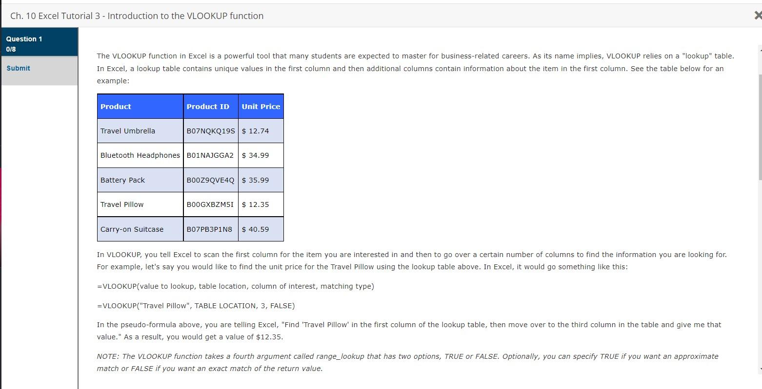
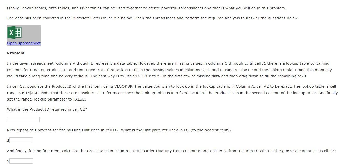
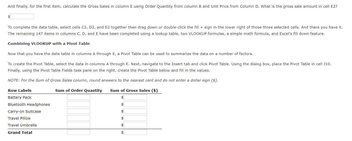
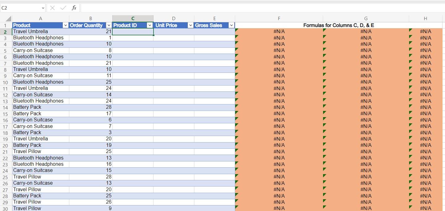
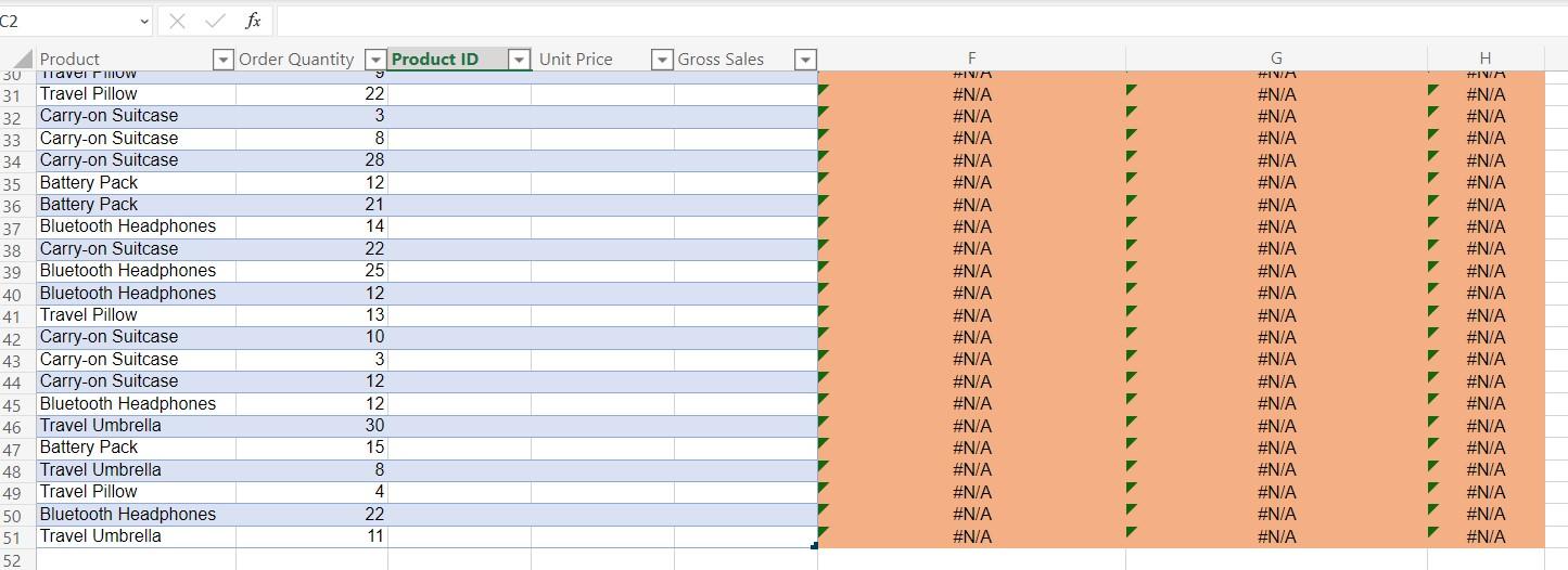
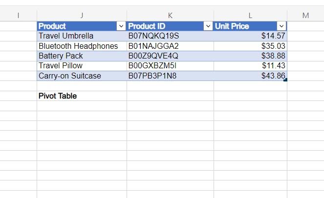
Ch. 10 Excel Tutorial 3 - Introduction to the VLOOKUP function Question 1 0/8 Submit The VLOOKUP function in Excel is a powerful tool that many students are expected to master for business-related careers. As its name implies, VLOOKUP relies on a "lookup" table. In Excel, a lookup table contains unique values in the first column and then additional columns contain information about the item in the first column. See the table below for an example: Product Travel Umbrella Battery Pack Travel Pillow Product ID Bluetooth Headphones B01NAJGGA2 $34.99 Carry-on Suitcase Unit Price B07NQKQ19S $12.74 B00Z9QVE4Q $ 35.99 B00GXBZM5I $ 12.35 B07PB3P1N8 $40.59 In VLOOKUP, you tell Excel to scan the first column for the item you are interested in and then to go over a certain number of columns to find the information you are looking for. For example, let's say you would like to find the unit price for the Travel Pillow using the lookup table above. In Excel, it would go something like this: =VLOOKUP(value to lookup, table location, column of interest, matching type) =VLOOKUP("Travel Pillow", TABLE LOCATION, 3, FALSE) In the pseudo-formula above, you are telling Excel, "Find 'Travel Pillow' in the first column of the lookup table, then move over to the third column in the table and give me that value." As a result, you would get a value of $12.35. NOTE: The VLOOKUP function takes a fourth argument called range_lookup that has two options, TRUE or FALSE. Optionally, you can specify TRUE if you want an approximate match or FALSE if you want an exact match of the return value. x Finally, lookup tables, data tables, and Pivot tables can be used together to create powerful spreadsheets and that is what you will do in this problem. The data has been collected in the Microsoft Excel Online file below. Open the spreadsheet and perform the required analysis to answer the questions below. X Open spreadsheet Problem In the given spreadsheet, columns A though E represent a data table. However, there are missing values in columns C through E. In cell J1 there is a lookup table containing columns for Product, Product ID, and Unit Price. Your first task is to fill in the missing values in columns C, D, and E using VLOOKUP and the lookup table. Doing this manually would take a long time and be very tedious. The best way is to use VLOOKUP to fill in the first row of missing data and then drag down to fill the remaining rows. In cell C2, populate the Product ID of the first item using VLOOKUP. The value you wish to look up in the lookup table is in Column A, cell A2 to be exact. The lookup table is cell range $J$1:$L$6. Note that these are absolute cell references since the look up table is in a fixed location. The Product ID is in the second column of the lookup table. And finally set the range_lookup parameter to FALSE. What is the Product ID returned in cell C2? Now repeat this process for the missing Unit Price in cell D2. What is the unit price returned in D2 (to the nearest cent)? $ And finally, for the first item, calculate the Gross Sales in column E using Order Quantity from column B and Unit Price from Column D. What is the gross sale amount in cell E2? $ And finally, for the first item, calculate the Gross Sales in column E using Order Quantity from column B and Unit Price from Column D. What is the gross sale amount in cell E2? $ To complete the data table, select cells C2, D2, and E2 together then drag down or double-click the fill + sign in the lower right of those three selected cells. And there you have it. The remaining 147 items in columns C, D, and E have been completed using a lookup table, two VLOOKUP formulas, a simple math formula, and Excel's fill down feature. Combining VLOOKUP with a Pivot Table Now that you have the data table in columns A through E, a Pivot Table can be used to summarize the data on a number of factors. To create the Pivot Table, select the data in columns A through E. Next, navigate to the Insert tab and click Pivot Table. Using the dialog box, place the Pivot Table in cell J10. Finally, using the Pivot Table Fields task pane on the right, create the Pivot Table below and fill in the values. NOTE: For the Sum of Gross Sales column, round answers to the nearest cent and do not enter a dollar sign ($). Sum of Order Quantity Sum of Gross Sales ($) $ Row Labels Battery Pack Bluetooth Headphones Carry-on Suitcase Travel Pillow Travel Umbrella Grand Total $ $ $ $ $ C2 A 7 8 X fx 1 Product 2 Travel Umbrella 3 Bluetooth Headphones 4 Bluetooth Headphones 5 Carry-on Suitcase 6 Bluetooth Headphones Bluetooth Headphones Travel Umbrella 9 Carry-on Suitcase 10 Bluetooth Headphones 11 Travel Umbrella 12 Carry-on Suitcase 13 Bluetooth Headphones 14 Battery Pack 15 Battery Pack 16 Carry-on Suitcase 17 Carry-on Suitcase 18 19 Battery Pack Travel Umbrella B Order Quantity 20 Battery Pack 21 Travel Pillow 22 Bluetooth Headphones 23 Bluetooth Headphones 24 Carry-on Suitcase 25 Travel Pillow 26 Carry-on Suitcase 27 Travel Pillow 28 Battery Pack 29 Travel Pillow 30 Travel Pillow 21 1 10 8 10 21 10 11 25 24 14 24 28 17 6 7 3 20 19 25 13 16 15 28 13 20 25 26 9 Product ID D Unit Price E Gross Sales F #N/A #N/A #N/A #N/A #N/A #N/A #N/A #N/A #N/A #N/A #N/A #N/A #N/A #N/A #N/A #N/A #N/A #N/A #N/A #N/A #N/A #N/A #N/A #N/A #N/A #N/A #N/A #N/A #N/A G Formulas for Columns C, D, & E #N/A #N/A #N/A #N/A #N/A #N/A #N/A #N/A #N/A #N/A #N/A #N/A #N/A #N/A #N/A #N/A #N/A #N/A #N/A #N/A #N/A #N/A #N/A #N/A #N/A #N/A #N/A #N/A #N/A #N/A #N/A #N/A #N/A #N/A #N/A #N/A #N/A #N/A #N/A #N/A #N/A #N/A #N/A H #N/A #N/A #N/A V #N/A #N/A #N/A #N/A #N/A #N/A #N/A #N/A #N/A #N/A #N/A #N/A C2 Product 30 Taver POW 31 Travel Pillow 32 Carry-on Suitcase 33 Carry-on Suitcase 34 Carry-on Suitcase 35 Battery Pack 36 Battery Pack 37 Bluetooth Headphones 38 Carry-on Suitcase 39 Bluetooth Headphones 40 Bluetooth Headphones 41 Travel Pillow 42 Carry-on Suitcase 43 Carry-on Suitcase 44 Carry-on Suitcase 45 Bluetooth Headphones 46 Travel Umbrella 47 Battery Pack 48 Travel Umbrella 49 Travel Pillow 50 Bluetooth Headphones 51 Travel Umbrella 52 Order Quantity 22 3 8 28 12 21 14 22 25 12 13 10 3 12 12 30 15 8 4 22 11 Product ID Unit Price Gross Sales F #IV/A #N/A #N/A #N/A #N/A #N/A #N/A #N/A #N/A #N/A #N/A #N/A #N/A #N/A #N/A #N/A #N/A #N/A #N/A #N/A #N/A #N/A G #IV/A #N/A #N/A #N/A #N/A #N/A #N/A #N/A #N/A #N/A #N/A #N/A #N/A #N/A #N/A #N/A #N/A #N/A #N/A #N/A #N/A #N/A #N/A #N/A #N/A #N/A #N/A #N/A #N/A #N/A #N/A #N/A #N/A #N/A #N/A #N/A #N/A #N/A #N/A #N/A #N/A #N/A ALA H #INA #N/A 1 Product Travel Umbrella Bluetooth Headphones Battery Pack Travel Pillow Carry-on Suitcase Pivot Table K Product ID B07NQKQ19S B01NAJGGA2 B00Z9QVE4Q B00GXBZM51 B07PB3P1N8 L Unit Price