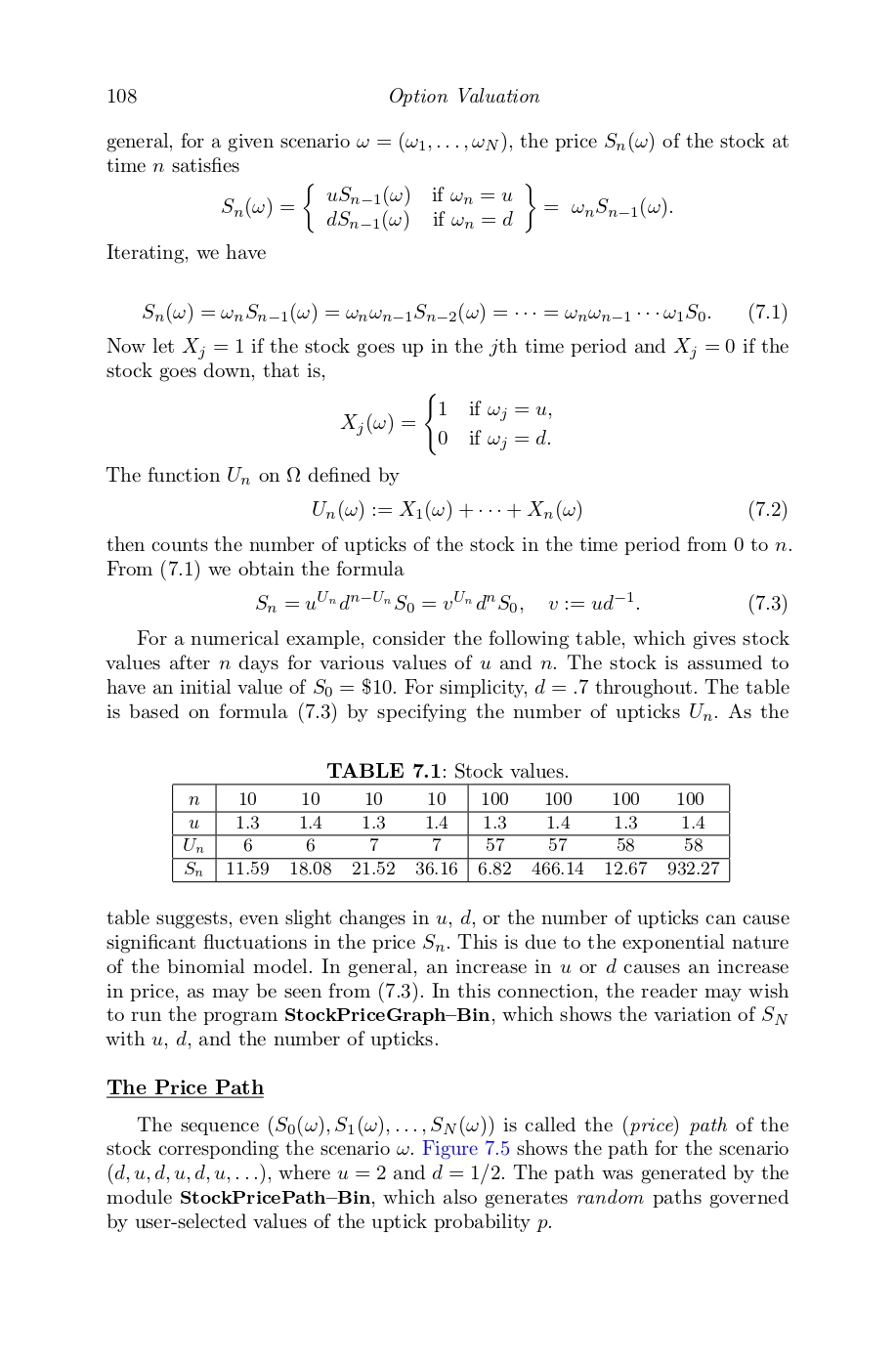
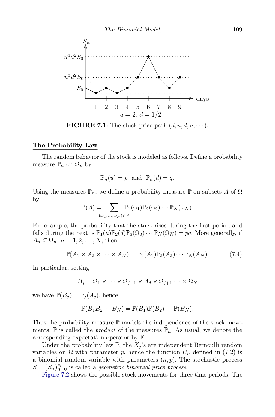
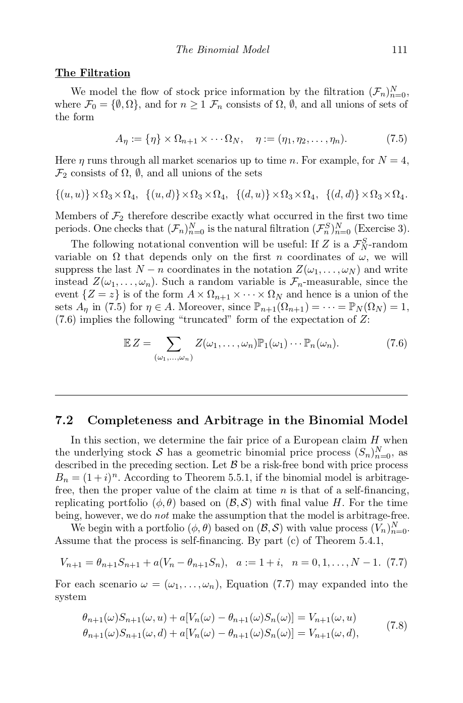
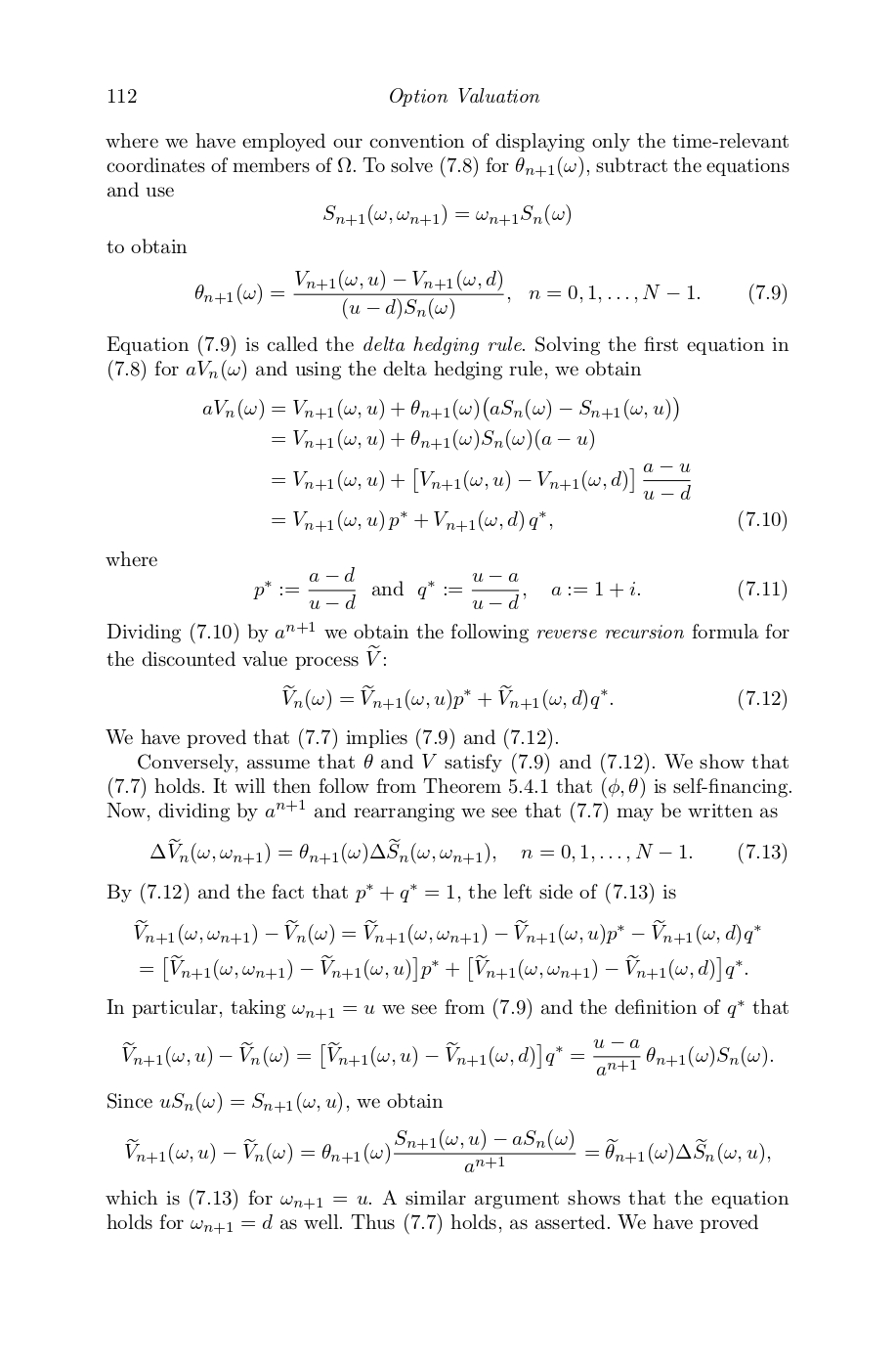
Chapter 7 The Binomial Model In this chapter, we construct the geometric binomial model for stock price movement and use the model to determine the value of a general European claim. An important consequence is the Cox-Ross-Rubinstein formula for the price of a call option. Formulas for path-dependent claims are given in the last section. The valuation techniques in this chapter are based on the notion of self-financing portfolio described in Chapter 5. 7.1 Construction of the Binomial Model Consider a (non-dividend paying) stock S with initial price So such that during each discrete time period the price changes either by a factor u with probability p or by a factor d with probability q := 1 -p, where 0 days 1 2 3 4 5 6 7 8 9 u = 2, d = 1/2 FIGURE 7.1: The stock price path (d, u, d, u, . . . ). The Probability Law The random behavior of the stock is modeled as follows. Define a probability measure Pn on 2n by Pn(u) = p and Pn(d) = q. Using the measures Pn, we define a probability measure P on subsets A of ? by P ( A) = _ PI ( W1 ) P 2 ( W2 ) .. . PN ( WN ) . ( W 1 ,... , WN ) EA For example, the probability that the stock rises during the first period and falls during the next is Pi(u)P2(d)P3(123) . . . PN(ON) = pq. More generally, if An C On, n = 1,2, ..., N, then P( A1 X A2 X . . . X AN) = P1(Al )P2(A2) . . . PN(AN). (7.4) In particular, setting Bj =01 x . .. x0j_1XAj X 2j+1 . . . x ON we have P(B;) = P;(A;), hence P(BIB2 . . . BN) = P(B1)P(B2) . . . P(BN). Thus the probability measure P models the independence of the stock move- ments. P is called the product of the measures Pn. As usual, we denote the corresponding expectation operator by E Under the probability law P, the Xj's are independent Bernoulli random variables on 2 with parameter p, hence the function Un defined in (7.2) is a binomial random variable with parameters (n, p). The stochastic process S = (Sn)n-o is called a geometric binomial price process. Figure 7.2 shows the possible stock movements for three time periods. The110 Option Valuation P - us So p u- So - u-dSo P - u-dSo ud So - ud- So So P u- dSo q p udSo -ud' So dSo P - ud- So q d' So - d' So FIGURE 7.2: 3-Step binomial tree. probabilities along the edges are conditional probabilities; specifically, P(Sn = ux | Sn-1 = x) = p and P(S, = da | Sn-1 = x) = q. Other conditional probabilities may be found by multiplying probabilities along edges and adding. For example, P(Sn = udx | Sn-2 = 2) = 2pq, since there are two paths leading from vertex a to vertex udx. 7.1.1 Example. The probability that the price of the stock at time n is larger than its initial price is found from (7.3) by observing that Sn > So () " d"> 1 Un> b:=; n lnd Ind - In u If d > 1, b is negative and P(S, > So) = 1. If d So) = _ P(Un = j) = > ()pig"-, j=m+1 j=m+1 where m := [b] is the greatest integer in b. The following table lists these probabilities for n = 100 and various values of u, d, and p. TABLE 7.2: Probabilities that S100 > So. P 50 .50 .50 .55 .55 .55 45 45 45 u 1.20 1.21 1.20 1.20 ) 1.21 1.20 1.20 1.21 1.20 d 80 .80 79 .80 80 .79 80 .80 79 P(S100 > So) .14 .24 .10 46 .62 .38 02 .04 .01 As in the case of stock prices, the probabilities are seen to be sensitive to slight variations of the parameters.The Binomial Model 111 The Filtration We model the flow of stock price information by the filtration (Fn)_ where Fo = {0, 0}, and for n 2 1 Fn consists of 2, 0, and all unions of sets of the form An : = {n} x Qntix .. . ON, n:= (11, 12, . .., nn). (7.5) Here n runs through all market scenarios up to time n. For example, for N = 4, F2 consists of , 0, and all unions of the sets {(u, u) }x93x24, {(u, d) }x93 x94, {(d, u)} x93 x94, {(d, d) } x83 x94. Members of F2 therefore describe exactly what occurred in the first two time periods. One checks that (Fn)_o is the natural filtration (F. )N n )n=0 (Exercise 3). The following notational convention will be useful: If Z is a Fi-random variable on S that depends only on the first n coordinates of w, we will suppress the last N - n coordinates in the notation Z(w1, . . ., WN) and write instead Z(w1, . ..,Wn). Such a random variable is Fn-measurable, since the event {Z = =} is of the form A X On+1 X . . . x 2x and hence is a union of the sets An in (7.5) for n E A. Moreover, since Pn+1(On+1) = . . . =PN(QN) = 1, (7.6) implies the following "truncated" form of the expectation of Z: E Z = > Z ( w1 , . . . , Wn) P1( w1 ) ... Pn( wn). (7.6) ( w1 ,..., Wr) 7.2 Completeness and Arbitrage in the Binomial Model In this section, we determine the fair price of a European claim H when the underlying stock S has a geometric binomial price process (S,)=0, as described in the preceding section. Let B be a risk-free bond with price process Bn = (1 + i)". According to Theorem 5.5.1, if the binomial model is arbitrage- free, then the proper value of the claim at time n is that of a self-financing, replicating portfolio (d, 0) based on (B, S) with final value H. For the time being, however, we do not make the assumption that the model is arbitrage-free. We begin with a portfolio (d, 0) based on (B, S) with value process (Vn)- Assume that the process is self-financing. By part (c) of Theorem 5.4.1, Vn+1 = On+1Sn+1 + a(Vn -On+1Sn), a := 1+i, n=0,1,.... N-1. (7.7) For each scenario w = (w1, . .., Wn), Equation (7.7) may expanded into the system Anti (w ) Sn+1 ( w, u) + alVn( w) - An+1( w) Sn(w)] = Vn+1(w, 2) Anti ( w) Snti( w, d ) + alVn(w) - An+1(w) Sn(w)] = Vn+1(w, d), (7.8 )112 Option Valuation where we have employed our convention of displaying only the time-relevant coordinates of members of 2. To solve (7.8) for On+1 (w), subtract the equations and use Snt1( w, wnt1 ) = wntISn(w) to obtain Anti(w) = Vn+1(w, u) - Vn+1(w, d) n = 0, 1, . .., N - 1. (7.9) (u - d) Sn(w) Equation (7.9) is called the delta hedging rule. Solving the first equation in (7.8) for aVn (w) and using the delta hedging rule, we obtain aVn ( w ) = VnitI(w, u) + Anti(w) ( asn ( w) - Sn+1 ( w , u ) ) = Vn+1 ( w, u) + On+1(w) Sn( w)(a-2) = Vn+1(w, u) + [Vn+1(w, 2) - Vn+1(w, d)] u _ d = Vnti(w, u) p* + Vn+1(w, d) q*, (7.10) where p* := a -d and q* := u - u - d u - a := 1+i. (7.11) Dividing (7.10) by anti we obtain the following reverse recursion formula for the discounted value process V: Vn ( w ) = Vn+1(w, u)p* + Vn+1( w, d) q*. (7.12) We have proved that (7.7) implies (7.9) and (7.12). Conversely, assume that 0 and V satisfy (7.9) and (7.12). We show that (7.7) holds. It will then follow from Theorem 5.4.1 that (o, 0) is self-financing. Now, dividing by ant and rearranging we see that (7.7) may be written as AVn ( w, wn+1) = On+1( w) ASn(w, wnt1), n =0,1, ..., N- 1. (7.13) By (7.12) and the fact that p* + q* = 1, the left side of (7.13) is Vn+1 ( w, wn+ 1 ) - Vn( w) = Vn+1 ( w, wn+1) - Vn+1(w, u)p* - Vn+1(w, d) q* = [ Vn+ 1 ( w, wn+1) - Vn+1( w, u) ]p* + [Vn+1( w, wn+1) - Vn+1( w, d) ]q*. In particular, taking wn+1 = u we see from (7.9) and the definition of q* that VnitI (w, 21) - Vn ( w) = [Vn+1 (w, 21) - Vn+1(w, d) ]q* = -nfi On+1(w) Sn(W). Since uSn(w) = Snti(w, u), we obtain Vnit1 ( w, 2 ) - Vn ( w) = On+1 (w) Sn+1 (w, 2) - an(W) = Anti( w) ASn(w, 2), an+1 which is (7.13) for wn+1 = u. A similar argument shows that the equation holds for wn+1 = d as well. Thus (7.7) holds, as asserted. We have provedQuestion 2: In the Geometric Binomial model of Chapter 7, calculate the following conditional probabilities: P(Sn = udx\\Sn-3 = x) and P(S, = d'x|Sn-3 = x)