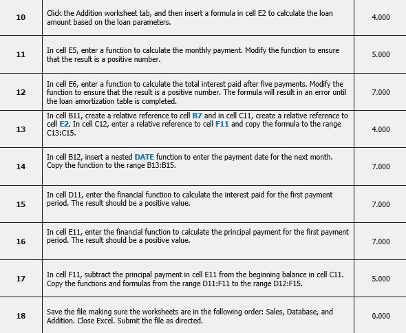
Click the Addition worksheet tab, and then insert a formula in cell E2 to calculate the loan amount based on the loan parameters. 4.000 In cell E5, enter a function to calculate the monthly payment. Modify the function to ensure that the result is a positive number 5.000 In cell E6, enter a function to calculate the total interest paid after five payments. Modify the function to ensure that the result is a positive number. The formula will result in an error until the loan amortization table is completed. 12 7.000 In cell B11, create a relative reference to cell B7 and in cell C11, create a relative reference to cell E2. In cell C12, enter a relative reference to cell F11 and copy the formula to the range C13:C15. 13 4.000 In cell B12, insert a nested DATE function to enter the payment date for the next month. 14 Copy the function to the range B13:B15 7.000 In cell D11, enter the financial function to calculate the interest paid for the first payment 15 period. The result should be a positive value. 7.000 In cell E11, enter the financial function to calculate the principal payment for the first payment 16 period. The result should be a positive value. 7.000 In cell F11, subtract the principal payment in cell E11 from the beginning balance in cell C11. Copy the functions and formulas from the range D11:F11 to the range D12:F15. 17 5.000 Save the file making sure the worksheets are in the following order: Sales, Database, and Addition. Close Excel. Submit the file as directed. 0.000 Click the Addition worksheet tab, and then insert a formula in cell E2 to calculate the loan amount based on the loan parameters. 4.000 In cell E5, enter a function to calculate the monthly payment. Modify the function to ensure that the result is a positive number 5.000 In cell E6, enter a function to calculate the total interest paid after five payments. Modify the function to ensure that the result is a positive number. The formula will result in an error until the loan amortization table is completed. 12 7.000 In cell B11, create a relative reference to cell B7 and in cell C11, create a relative reference to cell E2. In cell C12, enter a relative reference to cell F11 and copy the formula to the range C13:C15. 13 4.000 In cell B12, insert a nested DATE function to enter the payment date for the next month. 14 Copy the function to the range B13:B15 7.000 In cell D11, enter the financial function to calculate the interest paid for the first payment 15 period. The result should be a positive value. 7.000 In cell E11, enter the financial function to calculate the principal payment for the first payment 16 period. The result should be a positive value. 7.000 In cell F11, subtract the principal payment in cell E11 from the beginning balance in cell C11. Copy the functions and formulas from the range D11:F11 to the range D12:F15. 17 5.000 Save the file making sure the worksheets are in the following order: Sales, Database, and Addition. Close Excel. Submit the file as directed. 0.000