codes for this problem: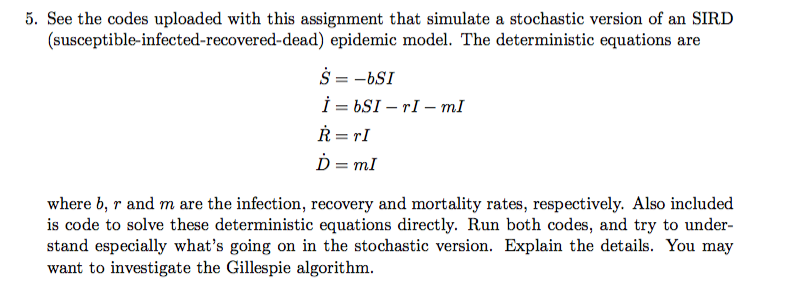

____________________________________________________________________________

CODE 1:

function sid_determ

% Simulation of a deterministic SIRD model using a differential % equation solver.

params.b = 0.02; % infection rate params.m = 0.1; % pathogen-induced mortality rate params.r = 0.3; % rate of recovery

initial.S = 50; % number of susceptible individuals initial.I = 1; % number of infected individuals initial.R = 0; % number of recovered individuals initial.D = 0; % number of dead people

end_time = 100; % end of simulation time span starting a 0

[t, y] = ode45(@(t, x) derivative(t, x, params), ... [0 end_time], ... [initial.S; initial.I; initial.R; initial.D], ... []); % extract result vectors outS = y(:,1); outI = y(:,2); outR = y(:,3); outD = y(:,4);

figure plot (t, y); grid xlabel ('time'); ylabel ('number of individuals'); legend('susceptible','infected','recovered','dead') set(gca,'fontsize',14)

function f = derivative (t, x, params) % Calculates the derivatives of the SIRD model. The output is a list with % the derivatives dS/dt, dI/dt and dR/dt at time t.

S = x(1); I = x(2); R = x(3); D = x(4); ds = -params.b * I * S; di = params.b * I * S - (params.m + params.r) * I; dr = params.r * I dd = params.m * I; f = [ds; di; dr; dd];

____________________________________________________________________

CODE 2:

function sid_run % Simulation of the stochastic SIR model

params.b = 0.02; % infection rate params.m = 0.1; % pathogen-induced mortality rate params.r = 0.3; % rate of recovery

initial.S = 50; % number of susceptible individuals initial.I = 1; % number of infected individuals initial.R = 0; % number of recovered individuals initial.D = 0; % number of dead people

end_time = 100; % end of simulation time span starting a 0 run_count = 200; % number of runs

result.time = []; % collects the time results result.S = []; % collects the S results result.I = []; % collects the I results result.R = []; % collects the R results result.D = []; % collects the D results

% simulate several stochastic SIR models and collect data for n=1:run_count out = sid (params, initial, end_time); result.time = [result.time out.time]; result.S = [result.S out.S]; result.I = [result.I out.I]; result.R = [result.R out.R]; result.D = [result.D out.D]; end

% extract unique times and the corresponding data [time, m, n] = unique(result.time); S = result.S(m); I = result.I(m); R = result.R(m); D = result.D(m);

% calculate running averages N = 50; % number of samples in the average j = 1; for i=1:N:length(time)-N+1 meanTime(j) = mean(time(i:i+N-1)); meanS(j) = mean(S(i:i+N-1)); meanI(j) = mean(I(i:i+N-1)); meanR(j) = mean(R(i:i+N-1)); meanD(j) = mean(D(i:i+N-1)); j = j + 1; end

% plot result figure plot (meanTime, meanS); hold plot (meanTime, meanI,'r'); plot (meanTime, meanR,'m'); plot (meanTime, meanD,'k'); grid xlabel ('time'); ylabel ('number of individuals'); legend('susceptible','infected','recovered','dead') set(gca,'fontsize',14)

_______________________________________________________________________

CODE 3:

function result = sid (params, initial, end_time)

% Simulation of the stochastic SIRD model: % % dS/dt = -b*S*I % dI/dt = b*S*I - m*I - r*I % dR/dt = r*I % dD/dt = m*I % % where % % S = susceptible, I = infected, R = recovered, D = dead % b = infection rate, r = recovery rate, m = mortality rate

state = initial; % holds the state variables S, I and R

result.time = []; % receives the time results result.S = []; % receives the S results result.I = []; % receives the I results result.R = []; % receives the R results result.D = []; % receives the D results

time = 0; while (time 0) % calculate process rates (probability/time) for current state a = rates(state, params);

% WHEN does the next process happen? %tau = exprnd(1/sum(probs)); % exprnd(mu) returns dist 1/mu*exp(-x/mu)

tau = -(1/sum(a))*log(rand(1)); % mu = 1/sum(a) %update time time = time + tau; % determine WHICH process happens after tau which = process(a); % update state switch which case 1 % S infected state.S = state.S - 1; state.I = state.I + 1; case 2 % I dies state.I = state.I - 1; state.D = state.D + 1; case 3 % I recovers state.I = state.I - 1; state.R = state.R + 1; end % store results result.time = [result.time time]; result.S = [result.S state.S]; result.I = [result.I state.I]; result.R = [result.R state.R]; result.D = [result.D state.D]; end

%--------------------------------------- function which = process (a) % Determines which process happens

r = rand * sum(a); which = 1; s = a(1); while (r > s) which = which + 1; s = s + a(which); end

%---------------------------------------- function a = rates (state, params) % Calculates process probabilities/time for given state and parameters

a(1) = params.b * state.S * state.I; % infection of susceptible a(2) = params.m * state.I; % death of infected a(3) = params.r * state.I; % recovery of infected

See the codes uploaded with this assignment that simulate a stochastic version of an SIRD (susceptible infected-recovered-dead) epidemic model. The deterministic equations are where b, r and m are the infection, recovery and mortality rates, respectively. Also included is code to solve these deterministic equations directly. Run both codes, and try to understand especially what's going on in the stochastic version. Explain the details. You may want to investigate the Gillespie algorithm