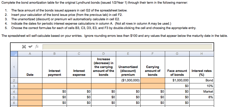
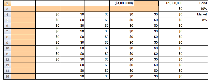
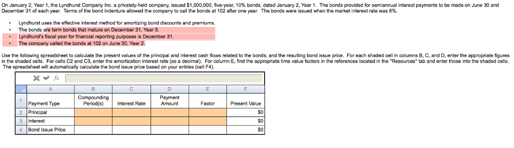
Complete the bond amortization table for the original Lyndhurst bonds (issued 1/2/Year 1) through their term in the following manner: The face amount of the bonds issued appears in cell G2 of the spreadsheet below. Insert your calculation of the bond issue price (from the previous tab) in cell F2. The unamortized (discount) or premium will automatically calculate in cell E2. Indicate the dates for periodic interest expense calculations in column A. (Not all rows in column A may be used.) Choose the correct formulas for each of cells B3, C3, D3, E3, and F3 by double-clicking the cell and choosing the appropriate entry. The spreadsheet will self-calculate based on your entries. Ignore rounding errors less than $100 and any values that appear below the maturity date in the table. On January 2. Year 1, the Lyndhurst Company Inc. a privately-held company, issued $1,000,000, five-year, 10% bonds, dated January 2. Year 1. The bonds provided for semiannual interest payments to be made on June 30 and December 31 of each year. Terms of the bond indenture allowed the company to call the bonds at 102 after one year. The bonds were issued when the market interest rate was 8%. Lyndhurst uses the effective interest method for amortizing bond discounts and premiums. The bonds are term bonds that mature on December 31. Year 5. Lyndhurst's fiscal year for financial reporting purposes is December 31 The company called the bonds at 102 on June 30, Year 2. Use the following spreadsheet to calculate the present values of the principal and interest cash flows related to the bonds, and the resulting bond issue price. For each shaded cell in columns B, C, and D, enter the appropriate figures in the shaded cells. For cells C2 and C3, enter the amortization Interest rate (as a decimal). For column E, find the appropriate time value factors in the references located in the 'Resources' tab and enter those into the shaded cells. The spreadsheet will automatically calculate the bond issue price based on your entries (cell F4). Complete the bond amortization table for the original Lyndhurst bonds (issued 1/2/Year 1) through their term in the following manner: The face amount of the bonds issued appears in cell G2 of the spreadsheet below. Insert your calculation of the bond issue price (from the previous tab) in cell F2. The unamortized (discount) or premium will automatically calculate in cell E2. Indicate the dates for periodic interest expense calculations in column A. (Not all rows in column A may be used.) Choose the correct formulas for each of cells B3, C3, D3, E3, and F3 by double-clicking the cell and choosing the appropriate entry. The spreadsheet will self-calculate based on your entries. Ignore rounding errors less than $100 and any values that appear below the maturity date in the table. On January 2. Year 1, the Lyndhurst Company Inc. a privately-held company, issued $1,000,000, five-year, 10% bonds, dated January 2. Year 1. The bonds provided for semiannual interest payments to be made on June 30 and December 31 of each year. Terms of the bond indenture allowed the company to call the bonds at 102 after one year. The bonds were issued when the market interest rate was 8%. Lyndhurst uses the effective interest method for amortizing bond discounts and premiums. The bonds are term bonds that mature on December 31. Year 5. Lyndhurst's fiscal year for financial reporting purposes is December 31 The company called the bonds at 102 on June 30, Year 2. Use the following spreadsheet to calculate the present values of the principal and interest cash flows related to the bonds, and the resulting bond issue price. For each shaded cell in columns B, C, and D, enter the appropriate figures in the shaded cells. For cells C2 and C3, enter the amortization Interest rate (as a decimal). For column E, find the appropriate time value factors in the references located in the 'Resources' tab and enter those into the shaded cells. The spreadsheet will automatically calculate the bond issue price based on your entries (cell F4)