complete this assignment and give a step by step solution on how to do it

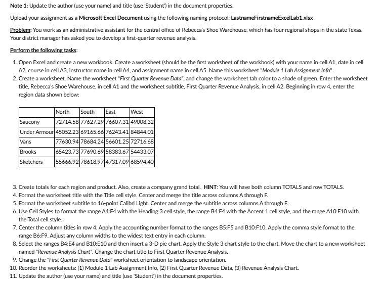
Note 1: Update the author (use your name) and title (use 'Student") in the document properties. Upload your assignment as a Microsoft Excel Document using the following naming protocol: LastnameFirstnameExcelLab1.xIsx Problem: You work as an administrative assistant for the central office of Rebecca's Shoe Warehouse, which has four regional shops in the state Texas. Your district manager has asked you to develop a first-quarter revenue analysis. Perform the following tasks: 1. Open Excel and create a new workbook. Create a worksheet (should be the first worksheet of the workbook) with your name in cell A1, date in cell A2, course in cell A3, instructor name in cell A4, and assignment name in cell A5. Name this worksheet "Module 1 Lab Assignment Info". 2. Create a worksheet. Name the worksheet "First Quarter Revenue Data", and change the worksheet tab color to a shade of green. Enter the worksheet title, Rebecca's Shoe Warehouse, in cell Al and the worksheet subtitle, First Quarter Revenue Analysis, in cell A2. Beginning in row 4, enter the region data shown below: North South East West Saucony 72714.58 77627.29 76607.31 49008.32 Under Armour 45052.23 69165.66 76243.41 84844.01 Vans 77630.94 78684.24 56601.25 72716.68 Brooks 65423.73 77690.69 58383.67 54433.07 Sketchers 55666.92 78618.97 47317.09 68594.40 3. Create totals for each region and product. Also, create a company grand total. HINT: You will have both column TOTALS and row TOTALS. 4. Format the worksheet title with the Title cell style. Center and merge the title across columns A through F. 5. Format the worksheet subtitle to 16-point Calibri Light. Center and merge the subtitle across columns A through F. 6. Use Cell Styles to format the range A4:F4 with the Heading 3 cell style, the range B4:F4 with the Accent 1 cell style, and the range A10:F10 with the Total cell style. 7. Center the column titles in row 4. Apply the accounting number format to the ranges B5:F5 and B10:F10. Apply the comma style format to the range B6:F9. Adjust any column widths to the widest text entry in each column. 8. Select the ranges B4:E4 and B10:E10 and then insert a 3-D pie chart. Apply the Style 3 chart style to the chart. Move the chart to a new worksheet named "Revenue Analysis Chart". Change the chart title to First Quarter Revenue Analysis. 9. Change the "First Quarter Revenue Data" worksheet orientation to landscape orientation. 10. Reorder the worksheets: (1) Module 1 Lab Assignment Info, (2) First Quarter Revenue Data, (3) Revenue Analysis Chart. 11. Update the author (use your name) and title (use 'Student") in the document properties