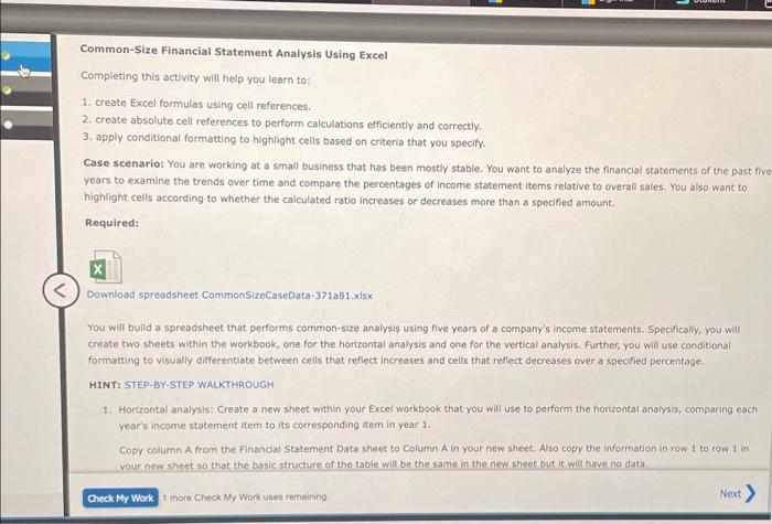
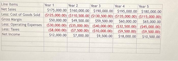
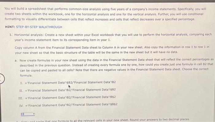
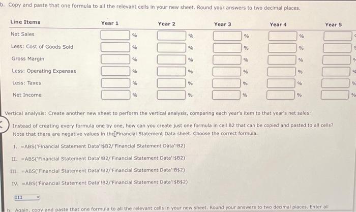
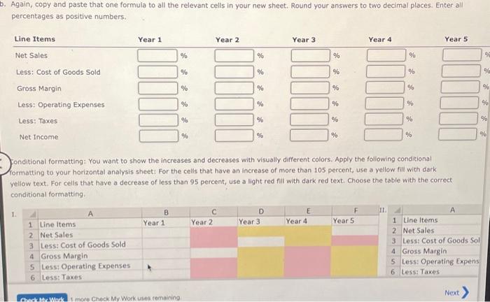
Completing this activity will help you learn to: 1. create Excel formulas using cell references. 2. create absolute cell references to perform caiculations efficiently and correctly: 3. apply conditional formatting to highlight cells based on criteria that you specify. Case scenario: You are working at a small business that has been mostly stable. You want to analyze the financial statements of the past fin years to examine the trends over time and compare the percentages of income statement items relative to overall sales. You aiso want to highlight cells according to whether the calculated ratio increases or decreases more than a specifed amount. Required: Downioad spreadsheet CommonsizeCaseData-371a81.xisx You will build a spreadsheet that performs common-size analysis using five years of a company's income statements. Specifically, you will create two sheets within the workbook, one for the horizontal analysis and one for the vertical analysis, Further, you will use conditional formatting to visually differentiate between cells that reflect increases and cells that reflect decreases over a specified percentage. HINT: STEP-BY-STEP WALKTHROUGH 1. Horizontal analysis: Create a new sheet within your Excel workbook that you will use to perform the horizontal analysis, comparing each year's income statement item to its corresponding item in year 1 . Copy column A from the Financial Statement Data sheet to Column A in your new sheet. Also copy the information in row 1 to row 1 in vour new sheet so that the bosic structure of the table will be the same in the new sheet but it wili have no data. \begin{tabular}{|l|r|r|r|r|r|} \hline Line Items & \multicolumn{1}{|c|}{ Year 1 } & Year 2 & Year 3 & \multicolumn{1}{|c|}{ Year 4 } & \multicolumn{1}{|c|}{ Year 5 } \\ \hline Net Sales & $175,000.00 & $160,000.00 & $190,000.00 & $195,000.00 & $180,000.00 \\ \hline Less: Cost of Goods Sold & ($125,000.00) & ($110,500.00 & ($130,500.00) & ($135,000.00) & ($115,000.00) \\ \hline Gross Margin & $50,000.00 & $49,500.00 & $59,500.00 & $60,000.00 & $65,000.00 \\ \hline Less: Operating Expenses & ($30,000.00) & ($35,000.00) & ($40,000.00) & ($32,500.00) & ($45,000.00) \\ \hline Less: Taxes & ($8,000.00) & ($7,500.00) & ($10,000.00) & ($9,500.00) & ($9,500.00) \\ \hline Net Income & $12,000.00 & $7,000.00 & $9,500.00 & $18,000.00 & $10,500.00 \\ \hline & & & & & \\ \hline & & & & & \\ \hline \end{tabular} will build a spreadsheet that performs common-size analysis using five years of a company's income statements. Specifically, you will ate two sheets within the workbook, one for the horizontal analysis and one for the vertical analysis. Further, you will use conditional matting to visually differentiate between cells that reflect increases and cells that reflect decreases over a specified percentage. NT: STEP-BY-STEP WALKTHROUGH 1. Horizontal analysis: Create a new sheet within your Excel workbook that you will use to perform the horizontal analysis, comparing each year's income statement item to its corresponding item in year 1. Copy column A from the Financial Statement Data sheet to Column A in your new sheet. Also copy the information in row 1 to row 1 in your new sheet so that the basic structure of the table will be the same in the new sheet but it will have no data. a. Now create formulas in your new sheet using the data in the Financial Statement Data sheet that will reflect the correct percentages a described in the previous question. Instead of creating every formula one by one, how could you create just one formula in cell B2 tha can be copied and pasted to all celis? Note that there are negative values in the Financial Statement Data sheet. Choose the correct formula. 1. ='Financial Statement Data'1\$B2/'Financial Statement Data'iB2 II. ='Financial Statement Data'1B2/FFinancial Statement Data'1582 III. ='Financial Statement Data'IB2/Financial Statement Data'IB\$2 IV. ='Financial Statement Data'lBz/'Financial Statement Data'I\$B\$2 Vertical analysis: Create another new sheet to perform the vertical analysis, comparing each year's item to that year's net sales: Instead of creating every formula one by one, how can you create just one formula in cell B2 that can be copied and posted to all cells? Note that there are negative values in thefinancial Statement Data sheet. Choose the correct formula. 1. =ABS('Financial Statement Data'ISB2/'Financial Statement Data'1B2) II. =ABS('Financial Statement Data'!82/'Financial Statement Data'15B2) III. =ABS('Financial Statement Data'IB2/'Financial Statement Data'iB $2 ) IV. =ABS('Financial Statement Data'lB2/'Financial Statement Data'I\$B\$2) Again, copy and paste that one formula to all the relevant cells in your new sheet. Round your answers to two decimal places. Enter all percentages as positive numbers. Fonditional formatting: You want to show the increases and decreases with visually different colors. Apply the folliowing conditional iormatting to your horizontal analysis sheet: For the ceils that have an increase of more than 105 percent, use a yellow fill with dark yellow text. For cells that have a decrease of less than 95 percent, use a light red fil with dark red text. Choose the table with the correct conditional formatting. Completing this activity will help you learn to: 1. create Excel formulas using cell references. 2. create absolute cell references to perform caiculations efficiently and correctly: 3. apply conditional formatting to highlight cells based on criteria that you specify. Case scenario: You are working at a small business that has been mostly stable. You want to analyze the financial statements of the past fin years to examine the trends over time and compare the percentages of income statement items relative to overall sales. You aiso want to highlight cells according to whether the calculated ratio increases or decreases more than a specifed amount. Required: Downioad spreadsheet CommonsizeCaseData-371a81.xisx You will build a spreadsheet that performs common-size analysis using five years of a company's income statements. Specifically, you will create two sheets within the workbook, one for the horizontal analysis and one for the vertical analysis, Further, you will use conditional formatting to visually differentiate between cells that reflect increases and cells that reflect decreases over a specified percentage. HINT: STEP-BY-STEP WALKTHROUGH 1. Horizontal analysis: Create a new sheet within your Excel workbook that you will use to perform the horizontal analysis, comparing each year's income statement item to its corresponding item in year 1 . Copy column A from the Financial Statement Data sheet to Column A in your new sheet. Also copy the information in row 1 to row 1 in vour new sheet so that the bosic structure of the table will be the same in the new sheet but it wili have no data. \begin{tabular}{|l|r|r|r|r|r|} \hline Line Items & \multicolumn{1}{|c|}{ Year 1 } & Year 2 & Year 3 & \multicolumn{1}{|c|}{ Year 4 } & \multicolumn{1}{|c|}{ Year 5 } \\ \hline Net Sales & $175,000.00 & $160,000.00 & $190,000.00 & $195,000.00 & $180,000.00 \\ \hline Less: Cost of Goods Sold & ($125,000.00) & ($110,500.00 & ($130,500.00) & ($135,000.00) & ($115,000.00) \\ \hline Gross Margin & $50,000.00 & $49,500.00 & $59,500.00 & $60,000.00 & $65,000.00 \\ \hline Less: Operating Expenses & ($30,000.00) & ($35,000.00) & ($40,000.00) & ($32,500.00) & ($45,000.00) \\ \hline Less: Taxes & ($8,000.00) & ($7,500.00) & ($10,000.00) & ($9,500.00) & ($9,500.00) \\ \hline Net Income & $12,000.00 & $7,000.00 & $9,500.00 & $18,000.00 & $10,500.00 \\ \hline & & & & & \\ \hline & & & & & \\ \hline \end{tabular} will build a spreadsheet that performs common-size analysis using five years of a company's income statements. Specifically, you will ate two sheets within the workbook, one for the horizontal analysis and one for the vertical analysis. Further, you will use conditional matting to visually differentiate between cells that reflect increases and cells that reflect decreases over a specified percentage. NT: STEP-BY-STEP WALKTHROUGH 1. Horizontal analysis: Create a new sheet within your Excel workbook that you will use to perform the horizontal analysis, comparing each year's income statement item to its corresponding item in year 1. Copy column A from the Financial Statement Data sheet to Column A in your new sheet. Also copy the information in row 1 to row 1 in your new sheet so that the basic structure of the table will be the same in the new sheet but it will have no data. a. Now create formulas in your new sheet using the data in the Financial Statement Data sheet that will reflect the correct percentages a described in the previous question. Instead of creating every formula one by one, how could you create just one formula in cell B2 tha can be copied and pasted to all celis? Note that there are negative values in the Financial Statement Data sheet. Choose the correct formula. 1. ='Financial Statement Data'1\$B2/'Financial Statement Data'iB2 II. ='Financial Statement Data'1B2/FFinancial Statement Data'1582 III. ='Financial Statement Data'IB2/Financial Statement Data'IB\$2 IV. ='Financial Statement Data'lBz/'Financial Statement Data'I\$B\$2 Vertical analysis: Create another new sheet to perform the vertical analysis, comparing each year's item to that year's net sales: Instead of creating every formula one by one, how can you create just one formula in cell B2 that can be copied and posted to all cells? Note that there are negative values in thefinancial Statement Data sheet. Choose the correct formula. 1. =ABS('Financial Statement Data'ISB2/'Financial Statement Data'1B2) II. =ABS('Financial Statement Data'!82/'Financial Statement Data'15B2) III. =ABS('Financial Statement Data'IB2/'Financial Statement Data'iB $2 ) IV. =ABS('Financial Statement Data'lB2/'Financial Statement Data'I\$B\$2) Again, copy and paste that one formula to all the relevant cells in your new sheet. Round your answers to two decimal places. Enter all percentages as positive numbers. Fonditional formatting: You want to show the increases and decreases with visually different colors. Apply the folliowing conditional iormatting to your horizontal analysis sheet: For the ceils that have an increase of more than 105 percent, use a yellow fill with dark yellow text. For cells that have a decrease of less than 95 percent, use a light red fil with dark red text. Choose the table with the correct conditional formatting